In dit labo passen we verschillende methoden toe om lineaire regressie parameters te schatten:
De closed form OLS oplossing
Vergelijking met scikit-learn, NumPy en statsmodels OLS implementaties
Gradient berekening met PyTorch autograd
Implementatie van Stochastic Gradient Descent
import matplotlib.pyplot as plt
import numpy as np
import pandas as pd
import seaborn as sns
import statsmodels.api as sm
import torch
from sklearn.datasets import fetch_california_housing
from sklearn.linear_model import LinearRegression
from sklearn.metrics import mean_squared_error, r2_score
from sklearn.preprocessing import StandardScaler

rng = np.random.default_rng(67)
torch.manual_seed(67)

plt.style.use("seaborn-v0_8-darkgrid")
sns.set_palette("husl")
Dataset California Housing 🌴
housing = fetch_california_housing(as_frame=True)
df = housing.frame

print(f"Dataset shape: {df.shape}")
print(f"\nFeatures: {housing.feature_names}")
print("\nFirst rows:")
display(df.head())

print("\nBasic statistics:")
display(df.describe())
Dataset shape: (20640, 9)
Features: ['MedInc', 'HouseAge', 'AveRooms', 'AveBedrms', 'Population', 'AveOccup', 'Latitude', 'Longitude']
First rows:
Basic statistics:
Design matrix
We werken met slechts twee predictor-variabelen:
MedInc: median income in block groupAveRooms: average number of rooms per household
De target variabele is MedHouseVal: median house value for California districts, expressed in hundreds of thousands of dollars ($100,000)
✍️
Hoe ziet de algemene matrix vorm van het model eruit?
✍️
Hoe ziet de parameter tensor er specifiek uit?
✍️
Hoe die de design/feature matrix er specifiek uit?
✍️
Hoe implementeren we deze tensors in Python?
x1 = "MedInc"  # Median income
x2 = "AveRooms"  # Average number of rooms
target = "MedHouseVal"  # Median house value

# Create feature matrix (without bias yet)
X_features = df[[x1, x2]].values
y = df[target].values

# Add bias term (column of ones) to create design matrix
X = np.column_stack([np.ones(X_features.shape[0]), X_features])

print(f"Design matrix X shape: {X.shape}")
print(f"Target vector y shape: {y.shape}")
print(f"\nFirst 5 rows of design matrix (bias, {x1}, {x2}):")
print(X[:5])
print("\nFirst 5 target values:")
print(y[:5])
Design matrix X shape: (20640, 3)
Target vector y shape: (20640,)
First 5 rows of design matrix (bias, MedInc, AveRooms):
[[1. 8.3252 6.98412698]
[1. 8.3014 6.23813708]
[1. 7.2574 8.28813559]
[1. 5.6431 5.8173516 ]
[1. 3.8462 6.28185328]]
First 5 target values:
[4.526 3.585 3.521 3.413 3.422]
✍️
# Create scaler and fit on features (without bias column)
scaler = StandardScaler()
X_features_scaled = scaler.fit_transform(X_features)

# Create design matrix with bias term
X_scaled = np.column_stack([np.ones(X_features_scaled.shape[0]), X_features_scaled])

# Scale target variable
y_mean = np.mean(y)
y_std = np.std(y)
y_scaled = (y - y_mean) / y_std
Conditienummer en Correlatie
✍️
Hoe is het gesteld met het conditienummer van de design matrix en de multicollineariteit bij de predictoren?
# Calculate condition number
condition_number = np.linalg.cond(X_scaled)
print(f"Condition number of design matrix: {condition_number:.2f}")
print("\nInterpretation:")
if condition_number < 10:
    print("- Excellent: Matrix is well-conditioned")
elif condition_number < 100:
    print("- Good: Matrix is reasonably well-conditioned")
elif condition_number < 1000:
    print("- Fair: Some numerical instability may occur")
else:
    print("- Poor: Matrix is ill-conditioned, results may be unreliable")
Condition number of design matrix: 1.40
Interpretation:
- Excellent: Matrix is well-conditioned
# Correlation analysis
correlation_data = pd.DataFrame(X_features_scaled, columns=[x1, x2])
correlation_data[target] = y_scaled

# Calculate correlation matrix
corr_matrix = correlation_data.corr()

print("Correlation matrix:")
display(corr_matrix)

# Visualize correlation matrix
plt.figure(figsize=(8, 6))
sns.heatmap(
    corr_matrix,
    annot=True,
    cmap="coolwarm",
    center=0,
    square=True,
    linewidths=1,
    cbar_kws={"shrink": 0.8},
)
plt.title("Correlation Heatmap")
plt.tight_layout()
plt.show()

# Check multicollinearity
predictor_correlation = corr_matrix.loc[x1, x2]
print(f"\nCorrelation between {x1} and {x2}: {predictor_correlation:.4f}")
print(f"Multicollinearity assessment: {'Low' if abs(predictor_correlation) < 0.7 else 'High'}")
Correlation matrix:
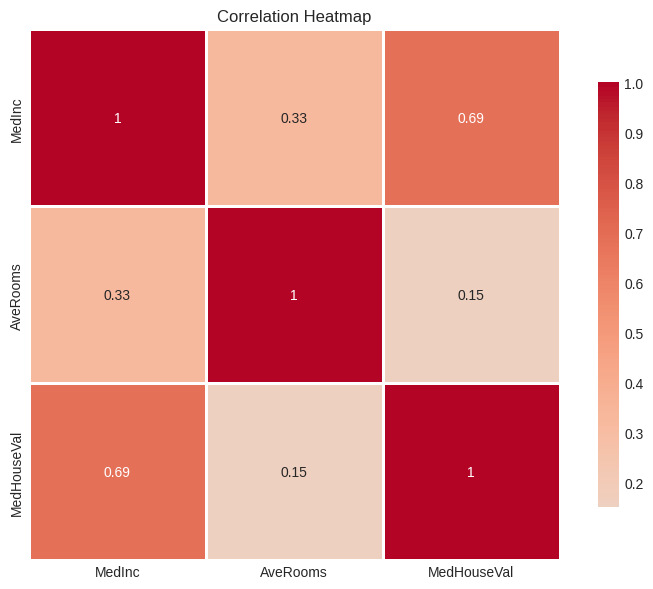
Correlation between MedInc and AveRooms: 0.3269
Multicollinearity assessment: Low
def closed_form_ols(X, y):
    """
    Compute OLS coefficients using the closed-form solution.

    Parameters
    ----------
    X : ndarray, shape (n_samples, n_features)
        Design matrix including bias term
    y : ndarray, shape (n_samples,)
        Target vector

    Returns
    -------
    beta : ndarray, shape (n_features,)
        Estimated coefficients
    """
    XtX = X.T @ X
    Xty = X.T @ y
    beta = np.linalg.inv(XtX) @ Xty
    return beta


# Calculate coefficients
beta_closed = closed_form_ols(X_scaled, y_scaled)

print("Closed-form OLS coefficients:")
print(f"  β₀ (bias):        {beta_closed[0]:.6f}")
print(f"  β₁ ({x1}):    {beta_closed[1]:.6f}")
print(f"  β₂ ({x2}): {beta_closed[2]:.6f}")

# Calculate predictions and metrics
y_pred_closed = X_scaled @ beta_closed
mse_closed = mean_squared_error(y_scaled, y_pred_closed)
r2_closed = r2_score(y_scaled, y_pred_closed)

print("\nModel performance:")
print(f"  MSE:  {mse_closed:.6f}")
print(f"  R²:   {r2_closed:.6f}")
Closed-form OLS coefficients:
β₀ (bias): 0.000000
β₁ (MedInc): 0.714787
β₂ (AveRooms): -0.081712
Model performance:
MSE: 0.520589
R²: 0.479411
Scikit-learn OLS
Hoe implementeren we OLS met scikit-learn?
# Scikit-learn LinearRegression
lr_sklearn = LinearRegression()
lr_sklearn.fit(X_features_scaled, y_scaled)

# Extract coefficients
beta_sklearn = np.array([lr_sklearn.intercept_, *lr_sklearn.coef_])

print("Scikit-learn OLS coefficients:")
print(f"  β₀ (bias):        {beta_sklearn[0]:.6f}")
print(f"  β₁ ({x1}):    {beta_sklearn[1]:.6f}")
print(f"  β₂ ({x2}): {beta_sklearn[2]:.6f}")

# Calculate metrics
y_pred_sklearn = lr_sklearn.predict(X_features_scaled)
mse_sklearn = mean_squared_error(y_scaled, y_pred_sklearn)
r2_sklearn = r2_score(y_scaled, y_pred_sklearn)

print("\nModel performance:")
print(f"  MSE:  {mse_sklearn:.6f}")
print(f"  R²:   {r2_sklearn:.6f}")
Scikit-learn OLS coefficients:
β₀ (bias): 0.000000
β₁ (MedInc): 0.714787
β₂ (AveRooms): -0.081712
Model performance:
MSE: 0.520589
R²: 0.479411
# NumPy least squares solution
beta_numpy, residuals, rank, s = np.linalg.lstsq(X_scaled, y_scaled, rcond=None)

print("NumPy lstsq OLS coefficients:")
print(f"  β₀ (bias):        {beta_numpy[0]:.6f}")
print(f"  β₁ ({x1}):    {beta_numpy[1]:.6f}")
print(f"  β₂ ({x2}): {beta_numpy[2]:.6f}")

# Calculate metrics
y_pred_numpy = X_scaled @ beta_numpy
mse_numpy = mean_squared_error(y_scaled, y_pred_numpy)
r2_numpy = r2_score(y_scaled, y_pred_numpy)

print("\nModel performance:")
print(f"  MSE:  {mse_numpy:.6f}")
print(f"  R²:   {r2_numpy:.6f}")
print("\nAdditional info:")
print(f"  Residual sum of squares: {residuals[0]:.6f}")
print(f"  Rank of design matrix: {rank}")
NumPy lstsq OLS coefficients:
β₀ (bias): 0.000000
β₁ (MedInc): 0.714787
β₂ (AveRooms): -0.081712
Model performance:
MSE: 0.520589
R²: 0.479411
Additional info:
Residual sum of squares: 10744.959552
Rank of design matrix: 3
Statsmodels OLS
Hoe implementeren we OLS met statsmodels?
# Statsmodels OLS
model_sm = sm.OLS(y_scaled, X_scaled)
results_sm = model_sm.fit()

# Extract coefficients
beta_statsmodels = results_sm.params

print("Statsmodels OLS coefficients:")
print(f"  β₀ (bias):        {beta_statsmodels[0]:.6f}")
print(f"  β₁ ({x1}):    {beta_statsmodels[1]:.6f}")
print(f"  β₂ ({x2}): {beta_statsmodels[2]:.6f}")

print("\nFull statistical summary:")
print(results_sm.summary())
Statsmodels OLS coefficients:
β₀ (bias): 0.000000
β₁ (MedInc): 0.714787
β₂ (AveRooms): -0.081712
Full statistical summary:
OLS Regression Results
==============================================================================
Dep. Variable: y R-squared: 0.479
Model: OLS Adj. R-squared: 0.479
Method: Least Squares F-statistic: 9502.
Date: Fri, 17 Oct 2025 Prob (F-statistic): 0.00
Time: 15:18:07 Log-Likelihood: -22550.
No. Observations: 20640 AIC: 4.511e+04
Df Residuals: 20637 BIC: 4.513e+04
Df Model: 2
Covariance Type: nonrobust
==============================================================================
coef std err t P>|t| [0.025 0.975]
------------------------------------------------------------------------------
const 4.753e-16 0.005 9.46e-14 1.000 -0.010 0.010
x1 0.7148 0.005 134.497 0.000 0.704 0.725
x2 -0.0817 0.005 -15.375 0.000 -0.092 -0.071
==============================================================================
Omnibus: 4804.179 Durbin-Watson: 0.692
Prob(Omnibus): 0.000 Jarque-Bera (JB): 12852.863
Skew: 1.250 Prob(JB): 0.00
Kurtosis: 5.949 Cond. No. 1.40
==============================================================================
Notes:
[1] Standard Errors assume that the covariance matrix of the errors is correctly specified.
Samenvatting
# Create comparison DataFrame
comparison_df = pd.DataFrame(
    {
        "Closed-form": beta_closed,
        "Scikit-learn": beta_sklearn,
        "NumPy lstsq": beta_numpy,
        "Statsmodels": beta_statsmodels,
    },
    index=["β₀ (bias)", f"β₁ ({x1})", f"β₂ ({x2})"],
)

print("Coefficient comparison:")
display(comparison_df)
Coefficient comparison:
Automatische differentiatie
PyTorch’s automatische differentiatie autograd berekent gradiënten automatisch. De bibliotheek is voornamelijk bedoeld voor gebruik bij neurale netwerken, maar hier kunnen we er al een eerste keer gebruik van maken om gradient descent te implementeren voor ons lineaire regressiemodel.
Hieronder eerst een demonstratie met een eenvoudig voorbeeld.
# Simple example: compute gradient of f(x) = x^2 + 3x + 5
print("Example: f(x) = x² + 3x + 5")
print("Analytical gradient: f'(x) = 2x + 3")

x = torch.tensor(2.0, requires_grad=True)
print(f"\nEvaluate at x = {x.item()}")

# Forward pass
f = x**2 + 3 * x + 5
print(f"f(x) = {f.item()}")

# Backward pass (compute gradient)
f.backward()
print(f"Computed gradient f'(x) = {x.grad.item()}")
print(f"Analytical gradient at x=2: 2(2) + 3 = {2 * 2 + 3}")
Example: f(x) = x² + 3x + 5
Analytical gradient: f'(x) = 2x + 3
Evaluate at x = 2.0
f(x) = 15.0
Computed gradient f'(x) = 7.0
Analytical gradient at x=2: 2(2) + 3 = 7
Hoe werkt automatische differentiatie?
In het bovenstaande voorbeeld zien we hoe PyTorch de gradiënt automatisch berekent:
Forward pass: We definiëren de functie
f = x² + 3x + 5en PyTorch houdt alle operaties bij in een computational graph.Backward pass: Bij het aanroepen van
f.backward()past PyTorch de som regel toe om de gradiënt te berekenen. Voor elke operatie in de graph kent PyTorch de afgeleide:Afgeleide van x²: 2x
Afgeleide van 3x: 3
Afgeleide van constante: 0
Resultaat: De gradiënt wordt opgeslagen in
x.grad. Bij x=2 vinden we f’(2) = 2(2) + 3 = 7.
Dit mechanisme is fundamenteel voor gradient descent: we kunnen complexe functies definiëren en PyTorch berekent automatisch de gradiënten die nodig zijn om de parameters te optimaliseren.
# Example with multiple variables
print("Example: f(x, y) = x²y + 3xy²")
print("∂f/∂x = 2xy + 3y²")
print("∂f/∂y = x² + 6xy")

x = torch.tensor(3.0, requires_grad=True)
y = torch.tensor(2.0, requires_grad=True)

print(f"\nEvaluate at x = {x.item()}, y = {y.item()}")

# Forward pass
f = x**2 * y + 3 * x * y**2
print(f"f(x, y) = {f.item()}")

# Backward pass
f.backward()
print("\nComputed gradients:")
print(f"  ∂f/∂x = {x.grad.item()}")
print(f"  ∂f/∂y = {y.grad.item()}")

print("\nAnalytical gradients at x=3, y=2:")
print(f"  ∂f/∂x = 2(3)(2) + 3(2)² = {2 * 3 * 2 + 3 * 2**2}")
print(f"  ∂f/∂y = (3)² + 6(3)(2) = {3**2 + 6 * 3 * 2}")
Example: f(x, y) = x²y + 3xy²
∂f/∂x = 2xy + 3y²
∂f/∂y = x² + 6xy
Evaluate at x = 3.0, y = 2.0
f(x, y) = 54.0
Computed gradients:
∂f/∂x = 24.0
∂f/∂y = 45.0
Analytical gradients at x=3, y=2:
∂f/∂x = 2(3)(2) + 3(2)² = 24
∂f/∂y = (3)² + 6(3)(2) = 45
Gradient Descent met autograd
✍️
# Parameter vector with initial values (zeros work well for standardized data)
b = torch.tensor([0.0, 0.0, 0.0], requires_grad=True, dtype=torch.float32)
print(f"Initial parameters: {b}")

# Design matrix
X_tensor = torch.tensor(X_scaled, dtype=torch.float32)

# Target vector
y_tensor = torch.tensor(y_scaled, dtype=torch.float32)

# Training loop
n_iterations = 1000
learning_rate = 0.01
loss_history = []

for i in range(n_iterations):
    # Forward pass: compute predictions
    y_pred = X_tensor @ b

    # Compute loss (Mean Squared Error)
    loss = torch.mean((y_tensor - y_pred) ** 2)

    # Backward pass: compute gradients (autograd!)
    loss.backward()  # Compute gradients via backpropagation

    # Update parameters
    with torch.no_grad():  # Disable gradient tracking for parameter update
        b -= learning_rate * b.grad

    # Zero gradients for next iteration (crucial!)
    b.grad.zero_()

    # Store loss for visualization
    loss_history.append(loss.item())

    if (i + 1) % 100 == 0 or i == 0:
        print(f"Iteration {i + 1}/{n_iterations}, Loss: {loss.item():.6f}")

# Extract learned parameters
print("\nFinal parameters: {b}")
print("\nComparison with closed-form OLS:")
print(f"  β₀: GD={b[0].item():.6f}, OLS={beta_closed[0]:.6f}")
print(f"  β₁: GD={b[1].item():.6f}, OLS={beta_closed[1]:.6f}")
print(f"  β₂: GD={b[2].item():.6f}, OLS={beta_closed[2]:.6f}")
Initial parameters: tensor([0., 0., 0.], requires_grad=True)
Iteration 1/1000, Loss: 1.000000
Iteration 100/1000, Loss: 0.536470
Iteration 200/1000, Loss: 0.521565
Iteration 300/1000, Loss: 0.520654
Iteration 400/1000, Loss: 0.520593
Iteration 500/1000, Loss: 0.520589
Iteration 600/1000, Loss: 0.520589
Iteration 700/1000, Loss: 0.520589
Iteration 800/1000, Loss: 0.520589
Iteration 900/1000, Loss: 0.520589
Iteration 1000/1000, Loss: 0.520589
Final parameters: {b}
Comparison with closed-form OLS:
β₀: GD=0.000000, OLS=0.000000
β₁: GD=0.714785, OLS=0.714787
β₂: GD=-0.081711, OLS=-0.081712
Stochastic Gradient Descent
🎯
# Mini-batch Stochastic Gradient Descent
print("Mini-batch Stochastic Gradient Descent")
print("=" * 50)
# Hyperparameters
batch_size = 256
n_epochs = 50
learning_rate_sgd = 0.01
# Initialize parameters
b_sgd = torch.tensor([0.0, 0.0, 0.0], requires_grad=True, dtype=torch.float32)
# Convert data to tensors (already done, but for clarity)
X_tensor = torch.tensor(X_scaled, dtype=torch.float32)
y_tensor = torch.tensor(y_scaled, dtype=torch.float32)
n_samples = X_tensor.shape[0]
n_batches = int(np.ceil(n_samples / batch_size))
print(f"Dataset size: {n_samples}")
print(f"Batch size: {batch_size}")
print(f"Batches per epoch: {n_batches}")
print(f"Number of epochs: {n_epochs}\n")
# Training loop
loss_history_sgd = []
epoch_losses = []
for epoch in range(n_epochs):
# Shuffle data at the start of each epoch
indices = torch.randperm(n_samples)
X_shuffled = X_tensor[indices]
y_shuffled = y_tensor[indices]
epoch_loss = 0.0
# Process mini-batches
for batch_idx in range(n_batches):
# Get batch data
start_idx = batch_idx * batch_size
end_idx = min(start_idx + batch_size, n_samples)
X_batch = X_shuffled[start_idx:end_idx]
y_batch = y_shuffled[start_idx:end_idx]
# Forward pass
y_pred_batch = X_batch @ b_sgd
# Compute loss for this batch
loss = torch.mean((y_batch - y_pred_batch) ** 2)
# Backward pass
loss.backward()
# Update parameters
with torch.no_grad():
b_sgd -= learning_rate_sgd * b_sgd.grad
# Zero gradients
b_sgd.grad.zero_()
# Track loss
epoch_loss += loss.item()
loss_history_sgd.append(loss.item())
# Average loss for the epoch
avg_epoch_loss = epoch_loss / n_batches
epoch_losses.append(avg_epoch_loss)
if (epoch + 1) % 10 == 0 or epoch == 0:
print(f"Epoch {epoch + 1}/{n_epochs}, Avg Loss: {avg_epoch_loss:.6f}")
print("\nTraining completed!")
print("\nFinal SGD parameters:")
print(f" β₀ (bias): {b_sgd[0].item():.6f}")
print(f" β₁ ({x1}): {b_sgd[1].item():.6f}")
print(f" β₂ ({x2}): {b_sgd[2].item():.6f}")
print("\nComparison with other methods:")
print(f" β₀: SGD={b_sgd[0].item():.6f}, GD={b[0].item():.6f}, OLS={beta_closed[0]:.6f}")
print(f" β₁: SGD={b_sgd[1].item():.6f}, GD={b[1].item():.6f}, OLS={beta_closed[1]:.6f}")
print(f" β₂: SGD={b_sgd[2].item():.6f}, GD={b[2].item():.6f}, OLS={beta_closed[2]:.6f}")
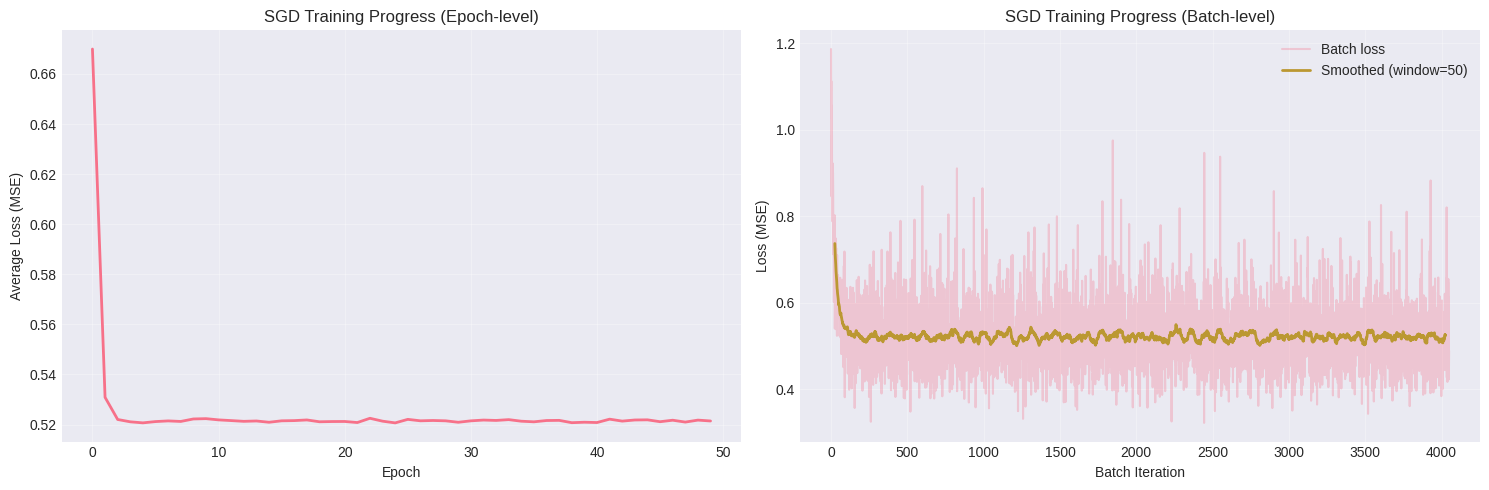
# Visualize training progress
fig, axes = plt.subplots(1, 2, figsize=(15, 5))
# Plot 1: Loss over epochs
axes[0].plot(epoch_losses, linewidth=2)
axes[0].set_xlabel("Epoch")
axes[0].set_ylabel("Average Loss (MSE)")
axes[0].set_title("SGD Training Progress (Epoch-level)")
axes[0].grid(True, alpha=0.3)
# Plot 2: Loss over all batch iterations (smoothed)
window = 50
if len(loss_history_sgd) > window:
smoothed_loss = pd.Series(loss_history_sgd).rolling(window=window, center=True).mean()
axes[1].plot(loss_history_sgd, alpha=0.3, label="Batch loss")
axes[1].plot(smoothed_loss, linewidth=2, label=f"Smoothed (window={window})")
axes[1].legend()
else:
axes[1].plot(loss_history_sgd, linewidth=2)
axes[1].set_xlabel("Batch Iteration")
axes[1].set_ylabel("Loss (MSE)")
axes[1].set_title("SGD Training Progress (Batch-level)")
axes[1].grid(True, alpha=0.3)
plt.tight_layout()
plt.show()
# Compare final predictions
y_pred_sgd = X_tensor @ b_sgd
mse_sgd = mean_squared_error(y_tensor.numpy(), y_pred_sgd.detach().numpy())
r2_sgd = r2_score(y_tensor.numpy(), y_pred_sgd.detach().numpy())
print("\nFinal SGD model performance:")
print(f" MSE: {mse_sgd:.6f}")
print(f" R²: {r2_sgd:.6f}")Mini-batch Stochastic Gradient Descent
==================================================
Dataset size: 20640
Batch size: 256
Batches per epoch: 81
Number of epochs: 50
Epoch 1/50, Avg Loss: 0.669930
Epoch 10/50, Avg Loss: 0.522375
Epoch 10/50, Avg Loss: 0.522375
Epoch 20/50, Avg Loss: 0.521220
Epoch 20/50, Avg Loss: 0.521220
Epoch 30/50, Avg Loss: 0.520929
Epoch 30/50, Avg Loss: 0.520929
Epoch 40/50, Avg Loss: 0.520946
Epoch 40/50, Avg Loss: 0.520946
Epoch 50/50, Avg Loss: 0.521442
Training completed!
Final SGD parameters:
β₀ (bias): 0.000466
β₁ (MedInc): 0.711527
β₂ (AveRooms): -0.072727
Comparison with other methods:
β₀: SGD=0.000466, GD=0.000000, OLS=0.000000
β₁: SGD=0.711527, GD=0.714785, OLS=0.714787
β₂: SGD=-0.072727, GD=-0.081711, OLS=-0.081712
Final SGD model performance:
  MSE:  0.520662
  R²:   0.479338
NumPy’s lstsq gebruikt SVD (Singular Value Decomposition) wat numeriek stabieler is dan directe matrix inversie.