Numerieke primitieven - Machine Learning Cursussen

Numerieke waarden worden in machine learning voorgesteld als één van de volgende wiskundige objecten: scalairen, vectoren, matrices of tensors.

Notatie¶

We volgen doorheen de cursus de notatieconventies in Goodfellow et al. (2016, xi-xiv).

Scalairen¶

Een scalaire waarde (of simpelweg “scalair”) is gewoon een enkelvoudig getal - in tegenstelling tot de andere objecten die een verzameling van meerdere getallen voorstellen.

We zullen ze in wiskundige notatie aanduiden met schuingedrukte kleine letters, bv. $s \in \mathbb{R}$ .

Ze hebben telkens een bepaald type:

natuurlijk: $\mathbb{N} = \{0, 1, 2, 3, ...\}$
geheel: $\mathbb{Z} = \{..., -3, -2, -1, 0, 1, 2, 3, ...\}$
rationaal: $\mathbb{Q} = \{..., -1.0, -0.5, 0, 0.5, 1, ...\}$
reëel: $\mathbb{R} = \mathbb{Q} \cup \{\pi, e, ...\}$
enz.

Vectoren¶

Een vector is een geordende reeks van getallen van éénzelfde type. Ieder individueel getal wordt geïdentificeerd door de index binnen de ordening (startend bij 1). Een vector duiden we in kleine letters en in het vet aan, bv. $\pmb{x}$ . Het eerste element duiden we aan met $x_1$ , het laatste met $x_n$ . Wanneer we de elementen expliciet willen voorstellen, gebruiken we een kolom met vierkante haakjes:

\pmb{x} = \begin{bmatrix} x_1 \cr \vdots \cr x_i \cr \vdots \cr x_n \end{bmatrix}

(1)

Om het type aan te duiden gebruiken we bv. $\pmb{x} \isin \mathbb{R}^n$ .
Vectoren laten ons toe om verschillende waarden van eenzelfde variabele samen voor te stellen. Dat maakt bijvoorbeeld in een programmeertaal als Python al een wereld van verschil.

import numpy as np
import plotly.graph_objects as go

# Without vectorization
a_1 = 5
a_2 = 8
a_3 = 12
# ...
a_100 = 3
print([a_1, a_2, a_3, a_100])

[5, 8, 12, 3]

# With vectorization
a = np.array([5, 8, 12, 3])
print(a)

[ 5  8 12  3]

We kunnen vectoren zien als de coördinaten van individuele punten in een $n$ -dimensionele ruimte.

# Define two points in 3D space as vectors
a = np.array([2, 3, 1])  # Point A: (2, 3, 1)
b = np.array([4, 1, 5])  # Point B: (4, 1, 5)

# Create traces for the 3D plot
traces = []

# Add origin point
traces.append(
    go.Scatter3d(
        x=[0],
        y=[0],
        z=[0],
        mode="markers",
        marker={"size": 8, "color": "black"},
        name="Origin (0,0,0)",
        showlegend=True,
    )
)

# Add point A
traces.append(
    go.Scatter3d(
        x=[a[0]],
        y=[a[1]],
        z=[a[2]],
        mode="markers+text",
        marker={"size": 8, "color": "red"},
        text=["A"],
        textposition="middle right",
        name=f"Point A {tuple(a)}",
        showlegend=True,
    )
)

# Add point B
traces.append(
    go.Scatter3d(
        x=[b[0]],
        y=[b[1]],
        z=[b[2]],
        mode="markers+text",
        marker={"size": 8, "color": "blue"},
        text=["B"],
        textposition="middle right",
        name=f"Point B {tuple(b)}",
        showlegend=True,
    )
)

# Add vector arrows from origin to points
# Vector A arrow
traces.append(
    go.Scatter3d(
        x=[0, a[0]],
        y=[0, a[1]],
        z=[0, a[2]],
        mode="lines",
        line={"color": "red", "width": 6},
        name="Vector A",
        showlegend=False,
    )
)

# Vector B arrow
traces.append(
    go.Scatter3d(
        x=[0, b[0]],
        y=[0, b[1]],
        z=[0, b[2]],
        mode="lines",
        line={"color": "blue", "width": 6},
        name="Vector B",
        showlegend=False,
    )
)

# Create the figure
fig = go.Figure(data=traces)

# Update layout
fig.update_layout(
    title="Two points in 3D space represented as vectors",
    scene={
        "xaxis_title": "X-axis",
        "yaxis_title": "Y-axis",
        "zaxis_title": "Z-axis",
        "camera": {"eye": {"x": 1.5, "y": 1.5, "z": 1.5}},
    },
    width=800,
    height=600,
)

# Show the plot
fig.show()

Loading...

Matrices¶

Wanneer we bijvoorbeeld niet 1 maar $m$ punten in een $n$ dimensionale ruimte willen weergeven, kunnen we een matrix notatie gebruiken: $\pmb{X} \isin \mathbb{R}^{mxn}$ . Een matrix is een geordende reeks van vectoren. We duiden ze aan in het vet met een hoofdletter, bv $\pmb{X}$ . Voor individuele elementen gebruiken we gewone hoofdletters, bv. $X_{2,4}$

\pmb{X} = \begin{bmatrix} X_{1,1} & \ldots & X_{1,j} & \ldots & X_{1,n} \cr \vdots & & \vdots & & \vdots \cr X_{i,1} & \ldots & X_{i,j} & \ldots & X_{i,n} \cr \vdots & & \vdots & & \vdots \cr X_{m,1} & \ldots & X_{m,j} & \ldots & X_{m,n} \end{bmatrix}

(2)

De rijen worden gevormd door rij-vectoren:

\pmb{x_i} = [X_{i, 1}, \ldots, X_{i, j}, \ldots, X_{i, n}]^T = \begin{bmatrix} X_{i, 1} \cr \vdots \cr X_{i, j} \cr \vdots \cr X_{i, n} \end{bmatrix}

(3)

De kolommen worden gevormd door kolom-vectoren:

\pmb{x_j} = \begin{bmatrix} X_{1, j} \cr \vdots \cr X_{i, j} \cr \vdots \cr X_{m, j} \end{bmatrix}

(4)

De notatie $\ldots^T$ duidt op transpositie tussen rijen en kolommen.

\pmb{X^T} = \begin{bmatrix} X_{1,1} & \ldots & X_{1, i} & \ldots & X_{1, m} \cr \vdots & & \vdots & & \vdots \cr X_{j, 1} & \ldots & X_{j,i} & \ldots & X_{j,m} \cr \vdots & & \vdots & & \vdots \cr X_{n,1} & \ldots & X_{n,i} & \ldots & X_{n,m} \end{bmatrix}

(5)

Matrices laten ons toe om verschillende waarden (rijen) van verschillende variabelen (kolommen) samen voor te stellen. Opnieuw: dat maakt een wereld van verschil uit als we dit willen programmeren.

# Without matrices
a_1_1 = 3
a_1_2 = 2
a_1_3 = 7
a_2_1 = 3
a_2_2 = 5
a_2_3 = 10
print([[a_1_1, a_1_2, a_1_3], [a_2_1, a_2_2, a_2_3]])

[[3, 2, 7], [3, 5, 10]]

a = np.array([[3, 2, 7], [3, 5, 10]])
print(a)
print(f"Shape of a: {a.shape}")

[[ 3  2  7]
 [ 3  5 10]]
Shape of a: (2, 3)

Tensors¶

Wanneer we het concept van een matrix uitbreiden naar een N-dimensionale grid van vectoren, spreken we van een tensor.

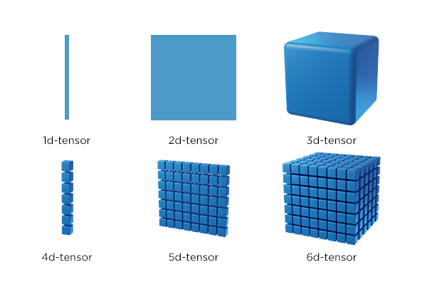
We kunnen dit illustreren aan de hand van beeld-data. Een RGB-afbeelding bestaat uit een verzameling pixels die geordend zijn in een 2-dimensionale grid. De dimensies worden bepaald door de resolutie; het aantal horizontale en verticale pixels. Iedere pixel is een vector met 3 waarden, overeenkomstig de channels: Rood, Groen, Blauw. Het gaat hier dus over een 3D tensor. De waarden zitten in een raster met een blok vorm (en dus niet in een vlak raster zoals bij matrices).

import matplotlib.pyplot as plt
from PIL import Image

with Image.open("../../../img/all_models_are_wrong.jpg") as img:
    plt.figure(figsize=(10, 6))
    plt.imshow(img)
    plt.axis("off")
    plt.show()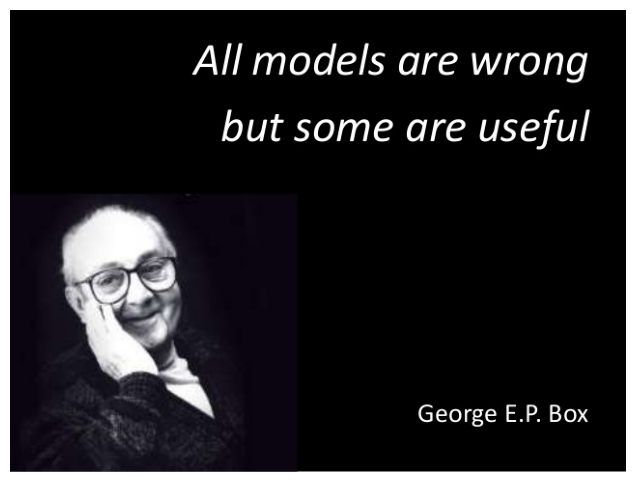

h, w, c = np.array(img).shape  # (height, width, channels)

print(f"Image dimensions: height={h}, width={w}, channels={c}")

Image dimensions: height=479, width=638, channels=3

# Sliced image
img_cropped = np.array(img)[-200:, :200, :]
plt.figure(figsize=(10, 6))
plt.imshow(img_cropped)
plt.axis("off")
plt.show()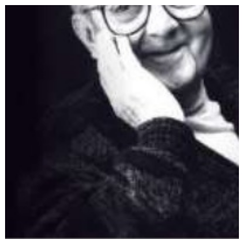

from matplotlib import patches

img_cropped_blue = img_cropped.copy()
img_cropped_blue[:, :, 2] = 255  # Set blue channel to max

# Create figure and axis
fig, ax = plt.subplots(figsize=(10, 6))
ax.imshow(img_cropped_blue)

# Add rectangle to indicate 10x10 region from bottom-left corner
# Rectangle coordinates: (x, y, width, height)
# Note: matplotlib uses (0,0) at top-left, so we need to adjust for bottom-left
height, width = img_cropped_blue.shape[:2]
rect = patches.Rectangle((0, height - 10), 10, 10, linewidth=2, edgecolor="red", facecolor="none")
ax.add_patch(rect)

ax.axis("off")
plt.show()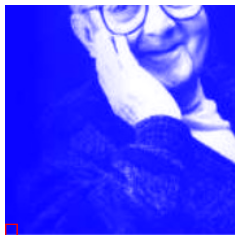

# 10x10x3 array from bottom-left corner
np.array(img)[-10, :10, :]

array([[12,  6, 18],
       [11,  5, 17],
       [10,  4, 16],
       [ 9,  3, 15],
       [ 9,  3, 15],
       [ 9,  3, 15],
       [ 9,  3, 15],
       [10,  4, 16],
       [10,  4, 16],
       [11,  5, 17]], dtype=uint8)

# Single pixel vector
np.array(img)[-100, 100, :]

array([27, 26, 31], dtype=uint8)

np.array(img.convert("CMYK")).shape

(479, 638, 4)