Informatietheorie - Machine Learning Cursussen

📚 ^[1]

Informatietheorie is een tak van de toegepaste wiskunde die draait om het kwantificeren van informatie in signalen. Dit domein werd oorspronkelijk ontwikkeld voor communicatie over ruis-gevoelige kanalen (zoals radiotransmissie), maar het is zeer aanwezig in machine learning om de mate van onzekerheid in probabiliteitsdistributies uit te drukken.

Self-Information¶

De self-information van een gebeurtenis $\text{x} = x$ kwantificeert hoeveel informatie die gebeurtenis bevat:

I(x) = -log P(x)

(1)

Deze formule voldoet aan drie intuïties waaraan een wiskundige uitdrukking van informatie moet voldoen:

Waarschijnlijke gebeurtenissen moeten een lagere informatiewaarde krijgen:
- Bij $P(x) = 1$ is er maximale zekerheid over de uitkomst; de self-information wordt $I(x) = -log(1) = 0$
- Bij $P(x) < 1$ stijgt de informatiewaarde: bv. $P(x) = 0.9 \Rightarrow I(x) = -log(0.9) \approx 0.11$
Onwaarschijnlijke gebeurtenissen moeten een hogere informatiewaarde krijgen:
- $P(x) = 0.1 \Rightarrow I(x) = -log(0.1) \approx 2.3$
- $P(x) = 0.01 \Rightarrow I(x) = -log(0.01) \approx 4.61$
Onafhankelijke gebeurtenissen moeten een additieve informatiewaarde hebben:
$x \perp y$
(2)

\begin{align} I(x, y) &= -log P(x, y) \cr &= -log P(x)P(y) \cr &= -log P(x) - log P(y) \cr &= I(x) + I(y) \end{align}

(3)

De eenheid van self-information wordt bepaald door de (arbitraire) basis van het logaritme:

$e$ bij het natuurlijke logaritme $-\text{ln} P(x)$ : de informatiewaarde wordt in nats uitgedrukt
$- \text{log}_2 P(x)$ : bits of shannons^[2]

Shannon entropie¶

De Shannon^[2] entropie meet de gemiddelde hoeveelheid informatie (of onzekerheid) op het niveau van de gehele kansverdeling:

H(\text{x}) = \mathbb{E}[I(\text{x})] = -\mathbb{E}[\log P(\text{x})] = -\sum_x P(x) \log P(x)

(5)

Voor continue variabelen wordt dit:

H(\text{x}) = -\int p(x) \log p(x) dx

(6)

Eigenschappen:

$H(\text{x}) \leq 0$
$H(\text{x}) = 0$ wanneer de verdeling deterministisch is (één uitkomst heeft $P(x)=1$ )
$H(\text{x})$ is maximaal voor een uniforme verdeling ( $P(x)=\frac{1}{k}$ in het discrete geval)

import matplotlib.pyplot as plt
import numpy as np

# Visualize entropy for binary distribution (coin flip)
# Create probability values from 0 to 1
p_values = np.linspace(0.001, 0.999, 1000)


# Calculate entropy for each probability value
# H(x) = -p*log(p) - (1-p)*log(1-p)
def binary_entropy(p):
    """Calculate entropy for binary distribution."""
    return -(p * np.log(p) + (1 - p) * np.log(1 - p))


H_values = binary_entropy(p_values)

# Create figure with two subplots
fig, axes = plt.subplots(1, 2, figsize=(14, 6))

# Left plot: Entropy curve
ax = axes[0]
ax.plot(p_values, H_values, "b-", linewidth=2.5)
ax.fill_between(p_values, H_values, alpha=0.2, color="blue")

# Mark maximum at p=0.5
max_entropy = binary_entropy(0.5)
ax.axvline(x=0.5, color="red", linestyle="--", linewidth=2, alpha=0.7)

# Mark some specific points
specific_points = [0.1, 0.3, 0.7, 0.9]
for p in specific_points:
    h = binary_entropy(p)
    ax.plot(p, h, "go", markersize=8, alpha=0.6)
    ax.annotate(
        f"p={p}\nH={h:.3f}",
        xy=(p, h),
        xytext=(10, 10),
        textcoords="offset points",
        fontsize=8,
        bbox={"boxstyle": "round,pad=0.3", "facecolor": "lightgreen", "alpha": 0.7},
        arrowprops={"arrowstyle": "->", "connectionstyle": "arc3,rad=0", "lw": 1},
    )

ax.set_xlabel("Probability P(x=heads)", fontsize=12, fontweight="bold")
ax.set_ylabel("Entropy H(x) [nats]", fontsize=12, fontweight="bold")
ax.set_title("Binary Distribution Entropy", fontsize=13, fontweight="bold")
ax.set_xlim(0, 1)
ax.set_ylim(0, 0.8)
ax.grid(alpha=0.3, linestyle="--")

# Add annotations for extreme cases
ax.text(
    0.05,
    0.05,
    "Deterministic\nP(heads=0)\nH≈0",
    fontsize=9,
    bbox={"boxstyle": "round", "facecolor": "lightcoral", "alpha": 0.7},
)
ax.text(
    0.82,
    0.05,
    "Deterministic\nP(heads=1)\nH≈0",
    fontsize=9,
    bbox={"boxstyle": "round", "facecolor": "lightcoral", "alpha": 0.7},
)
ax.text(
    0.5,
    0.75,
    "Maximum uncertainty\nUniform distribution",
    fontsize=9,
    ha="center",
    bbox={"boxstyle": "round", "facecolor": "yellow", "alpha": 0.8},
)

# Right plot: Bar chart showing distributions at specific points
ax = axes[1]
demo_probs = [0.1, 0.3, 0.5, 0.7, 0.9]
x_pos = np.arange(len(demo_probs))
width = 0.35

for i, p in enumerate(demo_probs):
    # Probability of heads and tails
    prob_heads = p
    prob_tails = 1 - p
    h = binary_entropy(p)

    # Create bars for this distribution
    ax.bar(
        i - width / 2,
        prob_heads,
        width,
        label="Heads" if i == 0 else "",
        color="steelblue",
        alpha=0.7,
        edgecolor="black",
    )
    ax.bar(
        i + width / 2,
        prob_tails,
        width,
        label="Tails" if i == 0 else "",
        color="coral",
        alpha=0.7,
        edgecolor="black",
    )

    # Add entropy value below
    ax.text(
        i,
        -0.15,
        f"H={h:.3f}",
        ha="center",
        fontsize=9,
        fontweight="bold",
        color="red" if p == 0.5 else "black",
    )

ax.set_ylabel("Probability", fontsize=12, fontweight="bold")
ax.set_xlabel("P(heads)", fontsize=12, fontweight="bold")
ax.set_title("Probability Distributions at Different P-values", fontsize=13, fontweight="bold")
ax.set_xticks(x_pos)
ax.set_xticklabels([f"{p:.1f}" for p in demo_probs])
ax.set_ylim(-0.2, 1.1)
ax.legend(fontsize=10, loc="upper right")
ax.grid(axis="y", alpha=0.3, linestyle="--")

# Highlight maximum entropy case
ax.axvspan(x_pos[2] - 0.4, x_pos[2] + 0.4, alpha=0.2, color="yellow")

plt.tight_layout()
plt.show()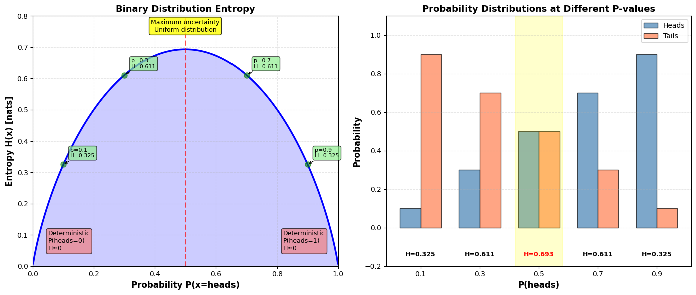

Kullback-Leibler (KL) divergentie¶

Als we twee aparte kansdistributies $P(x)$ en $Q(x)$ over dezelfde random variabele $\text{x}$ hebben, kunnen we meten hoe verschillend deze twee distributies zijn met de Kullback-Leibler divergentie:

D_{KL}(P \parallel Q) = \mathbb{E}_{x \sim P}\left[\log \frac{P(x)}{Q(x)}\right] = \mathbb{E}_{x \sim P}[\log P(x) - \log Q(x)]

(8)

Voor discrete variabelen:

D_{KL}(P \parallel Q) = \sum_x P(x) \log \frac{P(x)}{Q(x)}

(9)

Voor continue variabelen:

D_{KL}(P \parallel Q) = \int p(x) \log \frac{p(x)}{q(x)} dx

(10)

Eigenschappen:

$D_{KL}(P \parallel Q) \geq 0$ : Altijd positief
$D_{KL}(P \parallel Q) = 0 \Leftrightarrow P = Q$ : Nul bij identieke verdelingen
$D_{KL}(P \parallel Q) \neq D_{KL}(Q \parallel P)$ : ⚠️ Niet symmetrisch

from scipy import stats

# Define the distributions
x = np.linspace(-5, 10, 1000)

# P(x): Mixture of 2 Gaussians (true distribution)
# 60% from N(0, 1) and 40% from N(5, 1.5)
mu1, sigma1, weight1 = 0, 1, 0.6
mu2, sigma2, weight2 = 5, 1.5, 0.4

p_x = weight1 * stats.norm.pdf(x, mu1, sigma1) + weight2 * stats.norm.pdf(x, mu2, sigma2)

# Q(x): Single Gaussian (approximating distribution)
mu_q, sigma_q = 2.5, 2.5
q_x = stats.norm.pdf(x, mu_q, sigma_q)

# Calculate KL divergences
# D_KL(P||Q) - forward KL
# We need to be careful with numerical stability
epsilon = 1e-10
p_safe = np.where(p_x > epsilon, p_x, epsilon)
q_safe = np.where(q_x > epsilon, q_x, epsilon)

# Forward KL: D_KL(P||Q) = ∫ P(x) log(P(x)/Q(x)) dx
integrand_forward = p_safe * np.log(p_safe / q_safe)
kl_forward = np.trapezoid(integrand_forward, x)

# Reverse KL: D_KL(Q||P) = ∫ Q(x) log(Q(x)/P(x)) dx
integrand_reverse = q_safe * np.log(q_safe / p_safe)
kl_reverse = np.trapezoid(integrand_reverse, x)

# Create visualization
fig, axes = plt.subplots(2, 2, figsize=(15, 12))

# Top left: Show both distributions
ax = axes[0, 0]
ax.plot(x, p_x, "b-", linewidth=2.5, label="P(x): Mixture of 2 Gaussians", alpha=0.8)
ax.fill_between(x, p_x, alpha=0.2, color="blue")
ax.plot(x, q_x, "r-", linewidth=2.5, label="Q(x): Single Gaussian", alpha=0.8)
ax.fill_between(x, q_x, alpha=0.2, color="red")

# Mark the means
ax.axvline(mu1, color="blue", linestyle=":", alpha=0.5, linewidth=1.5)
ax.axvline(mu2, color="blue", linestyle=":", alpha=0.5, linewidth=1.5)
ax.axvline(mu_q, color="red", linestyle=":", alpha=0.5, linewidth=1.5)

ax.set_xlabel("x", fontsize=12, fontweight="bold")
ax.set_ylabel("Probability Density", fontsize=12, fontweight="bold")
ax.set_title("Two Probability Distributions", fontsize=13, fontweight="bold")
ax.legend(fontsize=11, loc="upper right")
ax.grid(alpha=0.3, linestyle="--")
ax.set_ylim(0, max(p_x.max(), q_x.max()) * 1.1)

# Top right: Forward KL - D_KL(P||Q)
ax = axes[0, 1]
# Highlight regions where P is high but Q is low
highlight_forward = np.where(p_x > q_x, integrand_forward, 0)
ax.fill_between(x, highlight_forward, alpha=0.4, color="orange", label="High penalty regions")
ax.plot(x, integrand_forward, "g-", linewidth=2, label="P(x)log(P(x)/Q(x))")
ax.axhline(0, color="black", linestyle="-", linewidth=0.5)

ax.set_xlabel("x", fontsize=12, fontweight="bold")
ax.set_ylabel("Integrand Value", fontsize=12, fontweight="bold")
ax.set_title(
    f"Forward KL: D$_{{KL}}$(P||Q) = {kl_forward:.4f} nats", fontsize=13, fontweight="bold"
)
ax.legend(fontsize=10)
ax.grid(alpha=0.3, linestyle="--")

# Add annotation
ax.text(
    0.05,
    0.95,
    "Penalizes when Q is low\nwhere P is high",
    transform=ax.transAxes,
    fontsize=10,
    verticalalignment="top",
    bbox={"boxstyle": "round", "facecolor": "wheat", "alpha": 0.8},
)

# Bottom left: Reverse KL - D_KL(Q||P)
ax = axes[1, 0]
# Highlight regions where Q is high but P is low
highlight_reverse = np.where(q_x > p_x, integrand_reverse, 0)
ax.fill_between(x, highlight_reverse, alpha=0.4, color="purple", label="High penalty regions")
ax.plot(x, integrand_reverse, "m-", linewidth=2, label="Q(x)log(Q(x)/P(x))")
ax.axhline(0, color="black", linestyle="-", linewidth=0.5)

ax.set_xlabel("x", fontsize=12, fontweight="bold")
ax.set_ylabel("Integrand Value", fontsize=12, fontweight="bold")
ax.set_title(
    f"Reverse KL: D$_{{KL}}$(Q||P) = {kl_reverse:.4f} nats", fontsize=13, fontweight="bold"
)
ax.legend(fontsize=10)
ax.grid(alpha=0.3, linestyle="--")

# Add annotation
ax.text(
    0.05,
    0.95,
    "Penalizes when Q is high\nwhere P is low",
    transform=ax.transAxes,
    fontsize=10,
    verticalalignment="top",
    bbox={"boxstyle": "round", "facecolor": "plum", "alpha": 0.8},
)

# Bottom right: Comparison of log ratios
ax = axes[1, 1]
log_ratio_forward = np.log(p_safe / q_safe)
log_ratio_reverse = np.log(q_safe / p_safe)

ax.plot(x, log_ratio_forward, "g-", linewidth=2, label="log(P(x)/Q(x))", alpha=0.7)
ax.plot(x, log_ratio_reverse, "m-", linewidth=2, label="log(Q(x)/P(x))", alpha=0.7)
ax.axhline(0, color="black", linestyle="--", linewidth=1)
ax.fill_between(
    x,
    0,
    log_ratio_forward,
    where=(log_ratio_forward > 0),
    alpha=0.2,
    color="green",
    label="P > Q regions",
)
ax.fill_between(
    x,
    0,
    log_ratio_reverse,
    where=(log_ratio_reverse > 0),
    alpha=0.2,
    color="magenta",
    label="Q > P regions",
)

ax.set_xlabel("x", fontsize=12, fontweight="bold")
ax.set_ylabel("Log Ratio", fontsize=12, fontweight="bold")
ax.set_title("Log Ratios: Asymmetry of KL Divergence", fontsize=13, fontweight="bold")
ax.legend(fontsize=10, loc="upper right")
ax.grid(alpha=0.3, linestyle="--")
ax.set_ylim(-5, 5)

plt.tight_layout()
plt.show()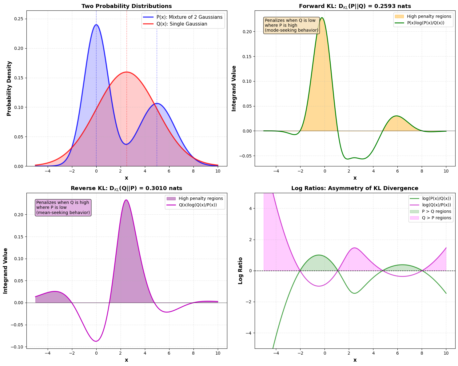

Cross-entropie¶

Een grootheid die nauw verwant is aan de KL divergentie is de cross-entropie:

H(P, Q) = H(P) + D_{KL}(P \parallel Q)

(11)

wat equivalent is aan:

H(P, Q) = -\mathbb{E}_{x \sim P}[\log Q(x)]

(12)

Voor discrete variabelen:

H(P, Q) = -\sum_x P(x) \log Q(x)

(13)

Voor continue variabelen:

H(P, Q) = -\int p(x) \log q(x) dx

(14)

Waarom cross-entropie in plaats van KL divergentie?

In machine learning wordt cross-entropie als loss functie gebruikt waarbij:

$P$ : de ware distributie van de trainingsdata voorstelt
$Q$ : de distributie van de modelvoorspellingen voorstelt

We willen de modelparameters en dus $Q$ zo kiezen, dat de cross-entropie minimaal wordt. Het minimaliseren van cross-entropie met betrekking tot $Q$ is equivalent aan het minimaliseren van de KL divergentie, omdat $Q$ niet deelneemt aan de $H(P)$ term in (11):

\arg\min_Q H(P, Q) = \arg\min_Q [H(P) + D_{KL}(P \parallel Q)] = \arg\min_Q D_{KL}(P \parallel Q)

(15)

De term $H(P)$ is een constante tijdens optimalisatie (hangt niet af van de modelparameters in $Q$ ), en valt dus weg bij het nemen van de afgeleide. We prefereren cross-entropie als loss functie omdat:

Berekenbaarheid: We kunnen $H(P, Q) = -\mathbb{E}_{x \sim P}[\log Q(x)]$ direct berekenen uit de trainingsdata, terwijl we voor KL divergentie ook $H(P) = -\mathbb{E}_{x \sim P}[\log P(x)]$ zouden moeten kennen, maar we kennen de ware distributie $P$ niet exact (we hebben alleen samples)
Eenvoud: Cross-entropie heeft een eenvoudigere implementatie - we hebben alleen de modelvoorspellingen $Q(x)$ en de labels nodig
Numerieke stabiliteit: De formule is rechtstreekser en minder gevoelig voor numerieke fouten

De volgende code demonstreert waarom beide loss functies tot dezelfde modelparameters leiden.

Voorbeelden in klassificatie

We zagen reeds het voorbeeld van cross-entropie loss functies in de context van

Binaire klassificatie (binary cross-entropy):
$\mathcal{L}_{BCE} = -\frac{1}{N}\sum_{i=1}^N [y_i \log \hat{y}_i + (1-y_i)\log(1-\hat{y}_i)]$
(16)
waarbij $y_i \in \{0,1\}$ de ware labels zijn en $\hat{y}_i \in (0,1)$ de voorspelde kansen.
Multi-class klassificatie (categorical cross-entropy):
$\mathcal{L}_{CCE} = -\frac{1}{N}\sum_{i=1}^N \sum_{c=1}^C y_{i,c} \log \hat{y}_{i,c}$
(17)
waarbij $y_{i,c}$ en $\hat{y}_{i,c}$ de ware en voorspelde kansen zijn voor klasse $c$ van voorbeeld $i$ .