Ordinary least squares - Machine Learning Cursussen

Hier passen we de closed form oplossing toe op de gesimuleerde koffieshop data.

\hat{\pmb{b}} = (\pmb{X}^T\pmb{X})^{-1}\pmb{X}^T\pmb{y}

(1)

Voor ons model met intercept en één predictor wordt de design matrix $\pmb{X}$ :

\pmb{X} = \begin{bmatrix} 1 & x_1 \\ 1 & x_2 \\ \vdots & \vdots \\ 1 & x_m \end{bmatrix}

(2)

# Data generation
sim = MonteCarloTipsSimulation(seed=42)

# Feature/design matrix X
n = len(sim.order_totals)
X = np.column_stack([np.ones(n), sim.order_totals])

# Closed form calculation

# Step 1: X^T X
XTX = X.T @ X

# Step 2: (X^T X)^(-1)
XTX_inv = np.linalg.inv(XTX)

# Step 3: X^T y
XTy = X.T @ sim.observed_tips

# Step 4: Final solution
beta_hat = XTX_inv @ XTy
b1_hat, b2_hat = beta_hat

print("\nEstimated parameters:")
print(f"b1_hat (intercept) = ${b1_hat:.3f}")
print(f"b2_hat (slope) = {b2_hat:.4f}")
print("\nTrue parameters:")
print(f"b1_true = ${sim.true_b1:.3f}")
print(f"b2_true = {sim.true_b2:.4f}")


Estimated parameters:
b1_hat (intercept) = $0.559
b2_hat (slope) = 0.1426

True parameters:
b1_true = $0.500
b2_true = 0.1500

# Visualization
plt.figure(figsize=(10, 6))
plt.scatter(
    sim.order_totals,
    sim.observed_tips,
    alpha=0.7,
    color="saddlebrown",
    s=60,
    edgecolor="white",
    linewidth=0.5,
    label="Observed tips",
)

# True relationship
plt.plot(
    sim.order_totals,
    sim.true_tips,
    "r--",
    linewidth=2,
    label=f"True relationship (${sim.true_b1:.2f} + {sim.true_b2:.1%} × order)",
)

# Estimated relationship
predicted_tips = b1_hat + b2_hat * sim.order_totals
plt.plot(
    sim.order_totals,
    predicted_tips,
    "b-",
    linewidth=2,
    label=f"Fitted relationship (${b1_hat:.2f} + {b2_hat:.1%} × order)",
)

plt.xlabel("Order Total ($)")
plt.ylabel("Tip Amount ($)")
plt.title("☕ Closed Form Solution - Fitted vs True Relationship")
plt.legend()
plt.grid(True, alpha=0.3)
plt.tight_layout()
plt.show()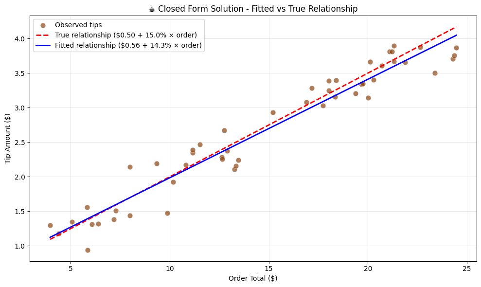

Voordeel¶

Optimale parameterwaarden op basis van SSE loss via één batch berekening.

Nadeel¶

De ordinary least squares oplossing heeft een belangrijke beperking: we moeten de matrix $(\pmb{X}^T\pmb{X})^{-1}$ kunnen berekenen. Dit vereist dat $\pmb{X}^T\pmb{X}$ volledig van rang is.

$\pmb{X}^T\pmb{X}$ is niet inverteerbaar (“singulier”) bij:

Perfecte multicollineariteit: Wanneer twee of meerdere features perfecte lineaire combinaties van elkaar zijn (of identiek aan elkaar).
Meer features dan observaties: Bij $M < N$ in $X$ , is $\pmb{X}^T\pmb{X}$ gegarandeerd singulier. De matrix $\pmb{X}^T\pmb{X}$ zal $N \times N$ zijn maar een rang hebben van maximaal $M < N$ .

Gevolgen:

Het systeem heeft ofwel geen unieke oplossing of oneindig veel oplossingen
Matrix inversie faalt numeriek
De parameters $\pmb{b}$ zijn niet uniek identificeerbaar

Zelf wanneer multicollineariteit niet perfect, maar wel substantieel is (en $\pmb{X}^T\pmb{X}$ inverteerbaar), is er een risico dat kleine veranderingen in de data tot grote verschillen in de parameterschattingen leiden en de onzekerheid over parameterschattingen zeer groot is.

Singulariteit of het risico op onstabiliteit kan gediagnosticeerd worden aan de hand van het zogeheten conditienummer.

Oplossingen:

Regularisatie (Ridge, Lasso): Het toevoegen van een penalty zoals $\lambda\pmb{I}$ (met $\lambda\geq0$ ) maakt $\pmb{X}^T\pmb{X} + \lambda\pmb{I}$ inverteerbaar.
Feature selectie: Verwijderen van redundante of collinear features.
Dimensionaliteitsreductie: PCA of andere technieken.
Pseudo-inverse: Het gebruik van de Moore-Penrose pseudo-inverse.
Iteratieve methoden: Gradient descent vereist geen matrix inversie.

Dit is waarom iteratieve gradiënt-gebaseerde optimalisatiemethoden vaak de voorkeur genieten in moderne machine learning, vooral voor modellen veel parameters.

Hieronder illustreren we de situatie bij $M < N$ .

rng = np.random.default_rng(123)
n_small = 3  # Only 3 observations
p = 4  # But we want to estimate 4 features

# Generate dataset
X_small = rng.standard_normal((n_small, p))
y_small = rng.standard_normal(n_small)

print(f"X_small shape: {X_small.shape}")
print(f"y_small shape: {y_small.shape}")

X_small shape: (3, 4)
y_small shape: (3,)

# Try closed form solution
XTX_small = X_small.T @ X_small

rank = np.linalg.matrix_rank(XTX_small)
print(f"Rank of X^T X: {rank} (should be {p})")
condition_number = np.linalg.cond(XTX_small)
print(f"Condition number of X^T X: {condition_number:.2e}")

try:
    XTX_inv_small = np.linalg.inv(XTX_small)
    beta_small = XTX_inv_small @ X_small.T @ y_small
    print(f"Estimated parameters: {beta_small}")

except Exception as e:
    print(f"❌ Error in matrix inversion: {e}")

Rank of X^T X: 3 (should be 4)
Condition number of X^T X: inf
Estimated parameters: [ 8.84011175 29.07666781 -5.22136417 -1.63398927]

Hoewel NumPy een inverse genereert, geeft het oneindige conditienummer aan dat $\pmb{X}^T\pmb{X}$ wel degelijk singulier is.

Hieronder illustreren we het probleem bij multicollineariteit

n = 10

# Feature 1: random numbers
x1 = rng.random(n)

# Feature 2: perfect linear combination of feature 1
x2 = 2 * x1 + 0.01  # Perfectly correlated

# Feature 3: constant (no information)
x3 = np.ones(n)

# Build design matrix with multicollinearity
X_multi = np.column_stack([x1, x2, x3])
y_multi = x1 + rng.random(n) * 0.1  # y depends mainly on x1

print(f"Correlation between x1 and x2: {np.corrcoef(x1, x2)[0, 1]:.6f}")

Correlation between x1 and x2: 1.000000

XTX_multi = X_multi.T @ X_multi

rank = np.linalg.matrix_rank(XTX_multi)
print(f"Rank of X^T X: {rank} (should be {p})")
condition_number = np.linalg.cond(XTX_multi)
print(f"Condition number of X^T X: {condition_number:.2e}")

try:
    XTX_inv_multi = np.linalg.inv(XTX_multi)
    beta_multi = XTX_inv_multi @ X_multi.T @ y_multi
    print(f"Estimated parameters: {beta_multi}")

except Exception as e:
    print(f"❌ Error in matrix inversion: {e}")

Rank of X^T X: 2 (should be 4)
Condition number of X^T X: 1.40e+16
Estimated parameters: [-2.47669566  0.75823902  0.07479962]

X_multi[0, 0] += 0.001  # Slightly perturb one value


XTX_multi = X_multi.T @ X_multi

rank = np.linalg.matrix_rank(XTX_multi)
print(f"Rank of X^T X: {rank} (should be {p})")
condition_number = np.linalg.cond(XTX_multi)
print(f"Condition number of X^T X: {condition_number:.2e}")

try:
    XTX_inv_multi = np.linalg.inv(XTX_multi)
    beta_multi = XTX_inv_multi @ X_multi.T @ y_multi
    print(f"Estimated parameters: {beta_multi}")

except Exception as e:
    print(f"❌ Error in matrix inversion: {e}")

Rank of X^T X: 3 (should be 4)
Condition number of X^T X: 3.39e+07
Estimated parameters: [-64.90113349  32.93863669  -0.24796529]

We zien hier geen oneindige, maar wel zeer grote conditienummers. Bovendien zorgt een heel kleine aanpassing van de data voor een grote verschuiving in de schattingen.