Perceptron - Machine Learning Cursussen

Tot nu toe hebben we het gehad over het lineaire regressiemodel en de verschillende manieren om de parameters te schatten. We hebben ook gezien hoe het logistische regressiemodel een uitbreiding is voor binaire klassificatie, waarbij een sigmoïde (S-vormige) functie (de link functie) lineaire predicties vertaalt naar het interval $[0, 1]$ . Het logistische regressiemodel is een specifiek geval van een generalized linear model.

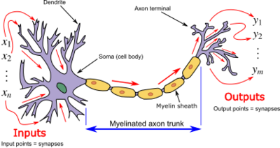
In deze sectie introduceren we het perceptron, de bouwsteen van neurale netwerken. Een perceptron is conceptueel zeer verwant aan generalized linear models. Het belangrijkste verschil zit in de terminologie: wat we bij GLMs een link functie noemen, wordt in de context van neurale netwerken een activatiefunctie genoemd.

Een perceptron is in feite een kunstmatig neuron dat de werking van een biologisch neuron nabootst:

De inputs $x_i$ zijn vergelijkbaar met signalen van andere neuronen
De gewichten $w_i$ bepalen de sterkte van elke verbinding
De activatiefunctie $\phi(z)$ bepaalt of het neuron “vuurt” (actief wordt)

import matplotlib.pyplot as plt
import numpy as np
import torch
from matplotlib.patches import Circle, FancyArrowPatch, Patch
from torch import nn, optim

from ml_courses.sim import generate_binary_tipping_data

Anatomie¶

Een perceptron bestaat uit:

Inputlaag (input layer): De feature waarden $x_1, x_2, \ldots, x_n$ (net zoals bij regressie)
Gewichten (weights): De parameters $w_1, w_2, \ldots, w_n$ (analoog aan de coëfficiënten $b_1, b_2, \ldots, b_n$ bij regressie)
Bias: De parameter $w_1$ (analoog aan het intercept $b_1$ bij regressie), waarbij $x_1=1$
Lineaire combinatie: $z = \sum_{i=1}^{n} w_i x_i = \pmb{x}^T\pmb{w}$
Activatiefunctie: $\phi(z)$ die de lineaire output niet-lineair transformeert
Output: De uiteindelijke predictie $\hat{y}^B = O(\phi(z))$

# Visualize the perceptron architecture
fig, ax = plt.subplots(figsize=(14, 8))
ax.set_xlim(0, 10)
ax.set_ylim(0, 10)
ax.axis("off")

# Define positions
input_y_positions = [7, 5.5, 4, 2.5]
input_x = 1.5
neuron_x = 5.5
output_x = 9

# Draw input nodes
input_nodes = []
for i, y_pos in enumerate(input_y_positions):
    if i == 0:
        # Bias node (special)
        circle = Circle(
            (input_x, y_pos), 0.35, color="lightcoral", ec="darkred", linewidth=2.5, zorder=3
        )
        ax.text(
            input_x,
            y_pos,
            "$1$",
            ha="center",
            va="center",
            fontsize=16,
            fontweight="bold",
            zorder=4,
        )
        ax.text(input_x - 0.9, y_pos, "bias", ha="center", va="center", fontsize=12, style="italic")
    else:
        # Regular input nodes
        circle = Circle(
            (input_x, y_pos), 0.35, color="lightblue", ec="darkblue", linewidth=2.5, zorder=3
        )
        ax.text(
            input_x,
            y_pos,
            f"$x_{i}$",
            ha="center",
            va="center",
            fontsize=16,
            fontweight="bold",
            zorder=4,
        )
        ax.text(input_x - 0.9, y_pos, f"input {i}", ha="center", va="center", fontsize=11)

    ax.add_patch(circle)
    input_nodes.append((input_x, y_pos))

# Draw neuron (perceptron)
neuron_center_y = 4.75
neuron = Circle(
    (neuron_x, neuron_center_y), 0.8, color="lightyellow", ec="orange", linewidth=3, zorder=3
)
ax.add_patch(neuron)

# Add sigma symbol and function label
ax.text(
    neuron_x,
    neuron_center_y + 0.15,
    "Σ",
    ha="center",
    va="center",
    fontsize=24,
    fontweight="bold",
    zorder=4,
)
ax.text(
    neuron_x,
    neuron_center_y - 0.4,
    "$z = h(\mathbf{x}, \mathbf{w})$",
    ha="center",
    va="center",
    fontsize=14,
    style="italic",
    zorder=4,
)
ax.text(
    neuron_x,
    neuron_center_y - 1.4,
    "perceptron",
    ha="center",
    va="center",
    fontsize=12,
    fontweight="bold",
)

# Draw output node
output_node = Circle(
    (output_x, neuron_center_y), 0.35, color="lightgreen", ec="darkgreen", linewidth=2.5, zorder=3
)
ax.add_patch(output_node)
ax.text(
    output_x,
    neuron_center_y,
    r"$\hat{y}$",
    ha="center",
    va="center",
    fontsize=16,
    fontweight="bold",
    zorder=4,
)
ax.text(
    output_x + 0.7, neuron_center_y, "output " + r"$\hat{o}$", ha="center", va="center", fontsize=11
)

# Draw connections from inputs to neuron with weights
for i, (x, y) in enumerate(input_nodes):
    arrow = FancyArrowPatch(
        (x + 0.35, y),
        (neuron_x - 0.8, neuron_center_y),
        arrowstyle="->",
        mutation_scale=20,
        linewidth=2,
        color="gray",
        alpha=0.7,
        zorder=1,
    )
    ax.add_patch(arrow)

    # Add weight labels
    mid_x = (x + neuron_x) / 2 - 0.3
    mid_y = (y + neuron_center_y) / 2
    ax.text(
        mid_x,
        mid_y,
        f"$w_{i}$",
        ha="center",
        va="bottom",
        fontsize=13,
        color="darkred" if i == 0 else "darkblue",
        fontweight="bold",
        bbox={"boxstyle": "round,pad=0.3", "facecolor": "white", "edgecolor": "none", "alpha": 0.8},
    )

# Draw connection from neuron to output
arrow = FancyArrowPatch(
    (neuron_x + 0.8, neuron_center_y),
    (output_x - 0.35, neuron_center_y),
    arrowstyle="->",
    mutation_scale=20,
    linewidth=2.5,
    color="darkgreen",
    zorder=2,
)
ax.add_patch(arrow)

# Add activation function label above arrow
ax.text(
    (neuron_x + output_x) / 2,
    neuron_center_y + 0.4,
    "activation",
    ha="center",
    va="bottom",
    fontsize=11,
    style="italic",
    color="darkgreen",
)

# Add formula annotations
# Linear combination
ax.text(
    neuron_x,
    neuron_center_y + 1.8,
    r"$z = w_0 + w_1x_1 + w_2x_2 + w_3x_3$",
    ha="center",
    va="center",
    fontsize=13,
    bbox={
        "boxstyle": "round,pad=0.5",
        "facecolor": "lightyellow",
        "edgecolor": "orange",
        "linewidth": 2,
    },
)

# Output formula
ax.text(
    output_x,
    neuron_center_y + 1.5,
    r"$\hat{y} = \phi(z)$",
    ha="center",
    va="center",
    fontsize=13,
    bbox={
        "boxstyle": "round,pad=0.4",
        "facecolor": "lightgreen",
        "edgecolor": "darkgreen",
        "linewidth": 2,
    },
)

# Add title
ax.text(5, 9.2, "Perceptron Architecture", ha="center", va="center", fontsize=18, fontweight="bold")

# Add legend/explanation box
legend_elements = [
    "Inputs: feature values (x₁, x₂, x₃) + bias (1)",
    "Weights: learnable parameters (w₀, w₁, w₂, w₃)",
    "Linear combination: z = Σ wᵢxᵢ",
    "Activation: φ(z) transforms z to output",
]
ax.text(
    5,
    0.7,
    "\n".join(legend_elements),
    ha="center",
    va="center",
    fontsize=10,
    bbox={
        "boxstyle": "round,pad=0.8",
        "facecolor": "wheat",
        "edgecolor": "gray",
        "linewidth": 1.5,
        "alpha": 0.9,
    },
)

plt.tight_layout()
plt.show()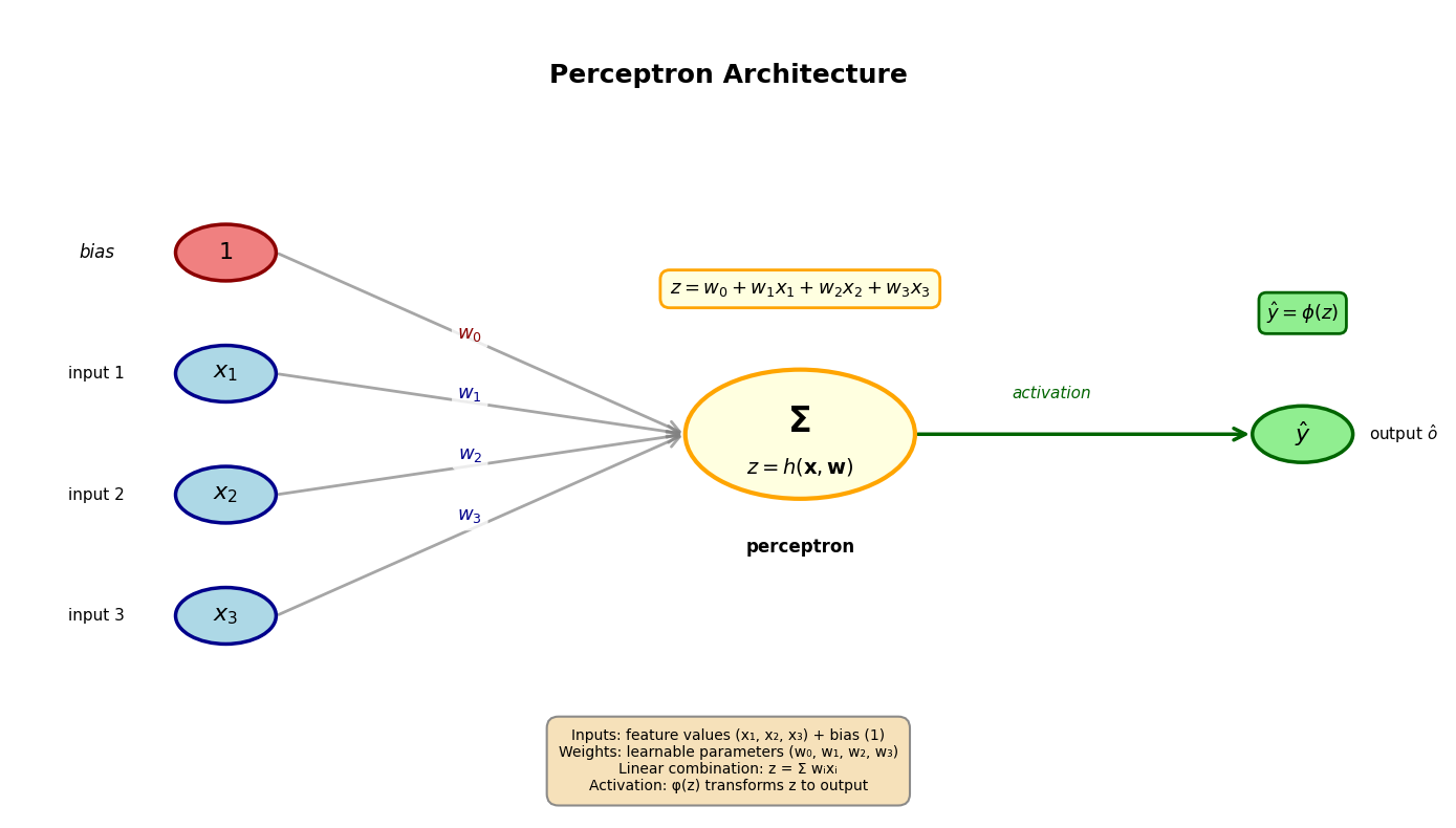

Activatiefuncties¶

De activatiefunctie $\phi(z)$ is cruciaal voor de werking van een perceptron. Ze vertaalt de lineaire combinatie van inputs en gewichten naar een output via een niet-lineaire transformatie die bepaalt of en in welke mate het perceptron actief wordt. Er bestaan verschillende varianten met verschillende eigenschappen. Hieronder bekijken we de meest gebruikelijke:

1. Logistische¶

De logistische functie is een S-vormige functie die we al kennen van het logistische regressiemodel:

\phi(z) = \sigma(z) = \frac{1}{1 + e^{-z}}

(1)

Bereik: $(0, 1)$
De lineaire combinatie $z$ noemen we ook =logits in deze context
Gebruik: Binaire klassificatie (output kan als probabiliteit geïnterpreteerd worden)

2. Tanh (Hyperbolische tangens)¶

Dit is ook een S-vormige functie die tussen -1 en 1 schaalt:

\phi(z) = \tanh(z) = \frac{e^z - e^{-z}}{e^z + e^{-z}}

(2)

Bereik: $(-1, 1)$
Voordeel: Zero-centered (gemiddelde output rond 0)

3. ReLU (Rectified Linear Unit)¶

ReLU is een piecewise linear functie en is de meest populaire activatiefunctie in moderne neurale netwerken:

\phi(z) = \max(0, z) = \begin{cases} z & \text{als } z > 0 \\ 0 & \text{als } z \leq 0 \end{cases}

(3)

Bereik: $[0, +\infty)$
Voordelen: Computationeel efficiënt, helpt vanishing gradients reduceren (zie verder)

4. GeLU (Gaussian Error Linear Unit)¶

GeLU is een continue variant van ReLU die steeds populairder wordt, vooral in de transformer modellen:

\phi(z) = z \cdot \Phi(z) \approx 0.5z\left(1 + \tanh\left[\sqrt{\frac{2}{\pi}}\left(z + 0.044715z^3\right)\right]\right)

(4)

waar $\Phi(z)$ de cumulatieve distributie van de standaard normaalverdeling of Gauss verdeling is.

Bereik: $(-\infty, +\infty)$
Voordelen: Continue differentieerbaar, niet-monotoon (kan negatieve waarden hebben)

4. Step function (Klassiek perceptron)¶

De originele activatiefunctie van het perceptron Rosenblatt (1958):

\phi(z) = \begin{cases} 1 & \text{als } z > 0 \\ 0 & \text{als } z \leq 0 \end{cases}

(5)

Bereik: $\{0, 1\}$
Probleem: Niet differentieerbaar, dus niet bruikbaar met gradient descent

# Visualize different activation functions
fig, axes = plt.subplots(2, 2, figsize=(14, 10))
axes = axes.flatten()

# Generate x values
x = np.linspace(-5, 5, 1000)

# 1. Logistic (Sigmoid)
ax = axes[0]
y_sigmoid = 1 / (1 + np.exp(-x))
ax.plot(x, y_sigmoid, "b-", linewidth=2.5, label="σ(z)")
ax.axhline(y=0, color="gray", linestyle="--", linewidth=0.8, alpha=0.7)
ax.axhline(y=0.5, color="gray", linestyle="--", linewidth=0.8, alpha=0.7)
ax.axhline(y=1, color="gray", linestyle="--", linewidth=0.8, alpha=0.7)
ax.axvline(x=0, color="gray", linestyle="--", linewidth=0.8, alpha=0.7)
ax.plot(0, 0.5, "ro", markersize=8, zorder=5)
ax.set_xlabel("z", fontsize=12, fontweight="bold")
ax.set_ylabel("φ(z)", fontsize=12, fontweight="bold")
ax.set_title("Logistic: φ(z) = 1/(1 + e⁻ᶻ)", fontsize=13, fontweight="bold")
ax.set_ylim(-0.2, 1.2)
ax.grid(True, alpha=0.3, linestyle=":", linewidth=0.5)
ax.legend(fontsize=11)
ax.text(
    2.5,
    0.1,
    "Range: (0, 1)",
    fontsize=10,
    bbox={"boxstyle": "round,pad=0.5", "facecolor": "lightblue", "alpha": 0.7},
)

# 2. Tanh
ax = axes[1]
y_tanh = np.tanh(x)
ax.plot(x, y_tanh, "g-", linewidth=2.5, label="tanh(z)")
ax.axhline(y=0, color="gray", linestyle="--", linewidth=0.8, alpha=0.7)
ax.axhline(y=1, color="gray", linestyle="--", linewidth=0.8, alpha=0.7)
ax.axhline(y=-1, color="gray", linestyle="--", linewidth=0.8, alpha=0.7)
ax.axvline(x=0, color="gray", linestyle="--", linewidth=0.8, alpha=0.7)
ax.plot(0, 0, "ro", markersize=8, zorder=5)
ax.set_xlabel("z", fontsize=12, fontweight="bold")
ax.set_ylabel("φ(z)", fontsize=12, fontweight="bold")
ax.set_title("Tanh: φ(z) = (eᶻ - e⁻ᶻ)/(eᶻ + e⁻ᶻ)", fontsize=13, fontweight="bold")
ax.set_ylim(-1.2, 1.2)
ax.grid(True, alpha=0.3, linestyle=":", linewidth=0.5)
ax.legend(fontsize=11)
ax.text(
    2.5,
    -0.8,
    "Range: (-1, 1)\nZero-centered",
    fontsize=10,
    bbox={"boxstyle": "round,pad=0.5", "facecolor": "lightgreen", "alpha": 0.7},
)

# 3. ReLU and GeLU
ax = axes[2]
y_relu = np.maximum(0, x)
# GeLU approximation: 0.5 * x * (1 + tanh(sqrt(2/pi) * (x + 0.044715 * x^3)))
y_gelu = 0.5 * x * (1 + np.tanh(np.sqrt(2 / np.pi) * (x + 0.044715 * x**3)))
ax.plot(x, y_relu, "r-", linewidth=2.5, label="ReLU: max(0, z)", alpha=0.8)
ax.plot(x, y_gelu, "orange", linewidth=2.5, linestyle="--", label="GeLU", alpha=0.8)
ax.axhline(y=0, color="gray", linestyle="--", linewidth=0.8, alpha=0.7)
ax.axvline(x=0, color="gray", linestyle="--", linewidth=0.8, alpha=0.7)
ax.plot(0, 0, "ro", markersize=8, zorder=5)
ax.set_xlabel("z", fontsize=12, fontweight="bold")
ax.set_ylabel("φ(z)", fontsize=12, fontweight="bold")
ax.set_title("ReLU & GeLU", fontsize=13, fontweight="bold")
ax.set_ylim(-0.5, 5.5)
ax.grid(True, alpha=0.3, linestyle=":", linewidth=0.5)
ax.legend(fontsize=10, loc="upper left")
ax.text(
    2.5,
    0.5,
    "ReLU: [0, ∞)\nGeLU: (-∞, ∞)",
    fontsize=10,
    bbox={"boxstyle": "round,pad=0.5", "facecolor": "lightcoral", "alpha": 0.7},
)

# 4. Step function
ax = axes[3]
x_step = np.linspace(-5, 5, 2)
y_step_neg = np.zeros_like(x_step[x_step < 0])
y_step_pos = np.ones_like(x_step[x_step >= 0])
ax.hlines(0, -5, 0, colors="purple", linewidth=2.5, label="step(z)")
ax.hlines(1, 0, 5, colors="purple", linewidth=2.5)
ax.plot(
    0, 0, "o", color="purple", markersize=8, markerfacecolor="white", markeredgewidth=2.5, zorder=5
)
ax.plot(0, 1, "o", color="purple", markersize=8, zorder=5)
ax.axhline(y=0, color="gray", linestyle="--", linewidth=0.8, alpha=0.7)
ax.axhline(y=1, color="gray", linestyle="--", linewidth=0.8, alpha=0.7)
ax.axvline(x=0, color="gray", linestyle="--", linewidth=0.8, alpha=0.7)
ax.set_xlabel("z", fontsize=12, fontweight="bold")
ax.set_ylabel("φ(z)", fontsize=12, fontweight="bold")
ax.set_title("Step: φ(z) = 1 if z > 0 else 0", fontsize=13, fontweight="bold")
ax.set_ylim(-0.2, 1.2)
ax.set_xlim(-5, 5)
ax.grid(True, alpha=0.3, linestyle=":", linewidth=0.5)
ax.legend(fontsize=11)
ax.text(
    2.5,
    0.1,
    "Range: {0, 1}\nNot differentiable",
    fontsize=10,
    bbox={"boxstyle": "round,pad=0.5", "facecolor": "plum", "alpha": 0.7},
)

plt.suptitle("Common Activation Functions", fontsize=16, fontweight="bold", y=1.00)
plt.tight_layout()
plt.show()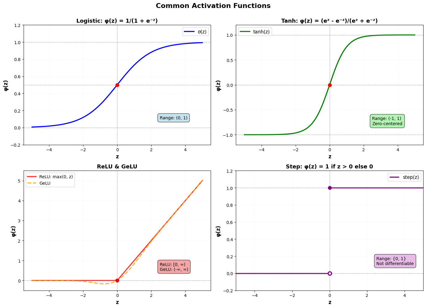

Analogie met logistische regressie¶

Als we bij een perceptron (a) voor de logistische activatiefunctie kiezen, en (b) de wiskundige notatie voor de volledige input $\pmb{X}$ data gebruiken, krijgen we enkel een verschil in benaming tussen de perceptron en logistische regressie formulering.

Logistische regressie:

\begin{align} \pmb{\hat{y}} &= \sigma(\pmb{X}\pmb{b}) \cr &= \frac{1}{1 + e^{-\pmb{X}\pmb{b}}} \end{align}

(6)

Perceptron

\begin{align} \pmb{\hat{y}} &= \phi(\pmb{X}\pmb{w}) \cr &= \frac{1}{1 + e^{-\pmb{X}\pmb{w}}} \end{align}

(7)

💡 We kunnen dus exact dezelfde gradient descent oplossing gebruiken!

Hieronder illustreren we dit, gebruikmakend van PyTorch en PyTorch’s automatische gradiëntberekening (autograd). We gebruiken dezelfde gesimuleerde data als in het logistische regressie voorbeeld.

# Generate the same tipping data as in the GLM notebook
X, y, metadata = generate_binary_tipping_data(n_customers=50, seed=42)

print("COFFEE SHOP TIPPING ANALYSIS (BINARY)")
print("=" * 50)
print(f"Dataset size: {len(y)} customers")
print(f"Order range: ${metadata['order_totals'].min():.2f} - ${metadata['order_totals'].max():.2f}")
print(f"Tippers: {metadata['n_tippers']} ({100 * metadata['tip_rate']:.1f}%)")
print(f"Non-tippers: {len(y) - metadata['n_tippers']} ({100 * (1 - metadata['tip_rate']):.1f}%)")
print("\nTrue model parameters:")
print(f"  Intercept (b₀): {metadata['true_b1']:.3f}")
print(f"  Slope (b₁):     {metadata['true_b2']:.3f}")
print(f"  P(tip) = σ({metadata['true_b1']:.2f} + {metadata['true_b2']:.2f} × order_total)")

COFFEE SHOP TIPPING ANALYSIS (BINARY)
==================================================
Dataset size: 50 customers
Order range: $3.96 - $24.46
Tippers: 43 (86.0%)
Non-tippers: 7 (14.0%)

True model parameters:
  Intercept (b₀): -2.000
  Slope (b₁):     0.250
  P(tip) = σ(-2.00 + 0.25 × order_total)

We trainen een perceptron met logistische activatiefunctie via gradient descent, gebruikmakend van PyTorch’s ingebouwde functionaliteit:

torch.nn.Linear: Een lineaire laag die $z = \pmb{x}^T\pmb{w} + b$ berekent
torch.nn.Sigmoid: De logistische activatiefunctie $\sigma(z)$
torch.nn.BCELoss: De binary cross-entropy loss functie
torch.optim.SGD: Stochastic gradient descent optimizer (met autograd!)

Deze aanpak is equivalent aan logistische regressie maar gebruikt de terminologie en tools van neurale netwerken.

# Define a simple perceptron model
# This is a single neuron: Linear layer + Sigmoid activation
class SimplePerceptron(nn.Module):
    """A simple perceptron model with sigmoid activation.

    This is a single neuron: Linear layer + Sigmoid activation.
    Note that PyTorch's nn.Linear already includes bias by default.
    """

    def __init__(self, input_dim):
        super().__init__()
        self.linear = nn.Linear(input_dim, 1)  # w^T x + b
        self.sigmoid = nn.Sigmoid()  # σ(z)

    def forward(self, x):
        """Perform forward pass through the perceptron.

        Args:
            x: Input tensor of shape (batch_size, input_dim)

        Returns
        -------
            Output tensor of shape (batch_size, 1) with sigmoid activation applied
        """
        z = self.linear(x)  # Linear combination
        y_hat = self.sigmoid(z)  # Apply activation
        return y_hat

# Convert numpy arrays to PyTorch tensors
X_torch = torch.tensor(X, dtype=torch.float32)
y_torch = torch.tensor(y, dtype=torch.float32).reshape(-1, 1)

# Initialize model
model = SimplePerceptron(input_dim=1)

# Define loss function and optimizer
criterion = nn.BCELoss()  # Binary Cross-Entropy Loss
optimizer = optim.SGD(model.parameters(), lr=0.01)  # Stochastic Gradient Descent

# Training loop
n_iterations = 50000
loss_history = []

for i in range(n_iterations):
    # Forward pass: compute predictions
    y_pred = model(X_torch)

    # Compute loss
    loss = criterion(y_pred, y_torch)

    # Backward pass: compute gradients (autograd!)
    optimizer.zero_grad()  # Clear previous gradients
    loss.backward()  # Compute gradients via backpropagation

    # Update parameters
    optimizer.step()

    # Store loss for visualization
    loss_history.append(loss.item())

    if (i + 1) % 10000 == 0:
        print(f"Iteration {i + 1}/{n_iterations}, Loss: {loss.item():.4f}")

# Extract learned parameters
learned_b0 = model.linear.bias.item()
learned_b1 = model.linear.weight.item()

print(f"\n{'=' * 60}")
print("RESULTS: PyTorch Perceptron (Logistic Activation)")
print(f"{'=' * 60}")
print("Learned parameters:")
print(f"  Intercept (b₀): {learned_b0:.3f}")
print(f"  Slope (b₁):     {learned_b1:.3f}")
print("\nTrue parameters:")
print(f"  Intercept (b₀): {metadata['true_b1']:.3f}")
print(f"  Slope (b₁):     {metadata['true_b2']:.3f}")
print(f"\nFinal loss: {loss_history[-1]:.4f}")
print(f"{'=' * 60}")

Iteration 10000/50000, Loss: 0.2763
Iteration 20000/50000, Loss: 0.2740
Iteration 30000/50000, Loss: 0.2738
Iteration 40000/50000, Loss: 0.2738
Iteration 50000/50000, Loss: 0.2738

============================================================
RESULTS: PyTorch Perceptron (Logistic Activation)
============================================================
Learned parameters:
  Intercept (b₀): -1.908
  Slope (b₁):     0.336

True parameters:
  Intercept (b₀): -2.000
  Slope (b₁):     0.250

Final loss: 0.2738
============================================================

⚠️ Beperking¶

Een enkelvoudig perceptron kan alleen lineair scheidbare klassen leren. De beslissingsgrens is altijd een rechte lijn (in 2D), een vlak (in 3D), of een hyper surface (in 4+D). Het klassieke voorbeeld van een niet-lineair scheidbaar probleem is de XOR-functie (exclusive OR).

# XOR problem
X_xor = np.array([[0, 0], [0, 1], [1, 0], [1, 1]], dtype=np.float32)
y_xor = np.array([0, 1, 1, 0], dtype=np.float32)  # XOR: output is 1 when inputs differ

# Convert to PyTorch tensors
X_xor_torch = torch.tensor(X_xor, dtype=torch.float32)
y_xor_torch = torch.tensor(y_xor, dtype=torch.float32).reshape(-1, 1)

# Train a perceptron on XOR using PyTorch
model_xor = SimplePerceptron(input_dim=2)
criterion_xor = nn.BCELoss()
optimizer_xor = optim.SGD(model_xor.parameters(), lr=0.1)

n_iterations_xor = 10000
for _ in range(n_iterations_xor):
    y_pred = model_xor(X_xor_torch)
    loss = criterion_xor(y_pred, y_xor_torch)
    optimizer_xor.zero_grad()
    loss.backward()
    optimizer_xor.step()

# Get predictions
with torch.no_grad():
    y_pred_xor_prob = model_xor(X_xor_torch).numpy().flatten()
    y_pred_xor = (y_pred_xor_prob >= 0.5).astype(int)

accuracy_xor = np.mean(y_pred_xor == y_xor)

print("XOR Problem:")
print(f"Perceptron accuracy: {accuracy_xor:.2%}")
print("\nPredictions vs True labels:")
for x, y_true, y_pred in zip(X_xor, y_xor, y_pred_xor, strict=True):
    status = "✓" if y_true == y_pred else "✗"
    print(f"  Input: {x} → True: {int(y_true)}, Predicted: {y_pred} {status}")

XOR Problem:
Perceptron accuracy: 50.00%

Predictions vs True labels:
  Input: [0. 0.] → True: 0, Predicted: 1 ✗
  Input: [0. 1.] → True: 1, Predicted: 1 ✓
  Input: [1. 0.] → True: 1, Predicted: 1 ✓
  Input: [1. 1.] → True: 0, Predicted: 1 ✗

# Visualize XOR problem and why it fails
fig, ax = plt.subplots(figsize=(10, 8))

# Create mesh for decision boundary
x_min, x_max = -0.5, 1.5
y_min, y_max = -0.5, 1.5
xx, yy = np.meshgrid(np.linspace(x_min, x_max, 200), np.linspace(y_min, y_max, 200))

# Predict on mesh using PyTorch model
with torch.no_grad():
    grid_points = torch.tensor(np.c_[xx.ravel(), yy.ravel()], dtype=torch.float32)
    Z = model_xor(grid_points).numpy().flatten()
    Z = Z.reshape(xx.shape)

# Plot contour
contour = ax.contourf(xx, yy, Z, levels=20, cmap="RdYlBu_r", alpha=0.6)
contour_line = ax.contour(xx, yy, Z, levels=[0.5], colors="black", linewidths=3)

# Plot XOR points
colors = ["blue" if y == 0 else "red" for y in y_xor]
for i, (x, y, color) in enumerate(zip(X_xor, y_xor, colors, strict=True)):
    marker = "o" if y == 0 else "s"
    ax.scatter(
        x[0],
        x[1],
        c=color,
        s=300,
        alpha=0.8,
        edgecolors="black",
        linewidth=3,
        marker=marker,
        zorder=5,
    )
    # Add labels
    ax.text(
        x[0],
        x[1],
        f"{int(y)}",
        ha="center",
        va="center",
        fontsize=16,
        fontweight="bold",
        color="white",
        zorder=6,
    )

# Add colorbar
cbar = plt.colorbar(contour, ax=ax)
cbar.set_label("P(y=1|x)", fontsize=11, fontweight="bold")

# Labels and styling
ax.set_xlabel("$x_1$", fontsize=13, fontweight="bold")
ax.set_ylabel("$x_2$", fontsize=13, fontweight="bold")
ax.set_title("XOR Problem: Not Linearly Separable", fontsize=15, fontweight="bold")
ax.set_xlim(x_min, x_max)
ax.set_ylim(y_min, y_max)
ax.grid(True, alpha=0.3, linestyle=":", linewidth=0.5)

# Add legend
legend_elements = [
    Patch(facecolor="blue", edgecolor="black", label="Class 0 (circle)"),
    Patch(facecolor="red", edgecolor="black", label="Class 1 (square)"),
]
ax.legend(handles=legend_elements, fontsize=11, loc="upper right")

# Add explanation text
explanation = (
    "No single straight line can separate\n"
    "the two classes correctly!\n"
    f"Best accuracy achieved: {accuracy_xor:.0%}"
)
ax.text(
    0.5,
    -0.35,
    explanation,
    ha="center",
    va="top",
    fontsize=11,
    bbox={
        "boxstyle": "round,pad=0.8",
        "facecolor": "yellow",
        "edgecolor": "black",
        "linewidth": 2,
        "alpha": 0.9,
    },
)

plt.tight_layout()
plt.show()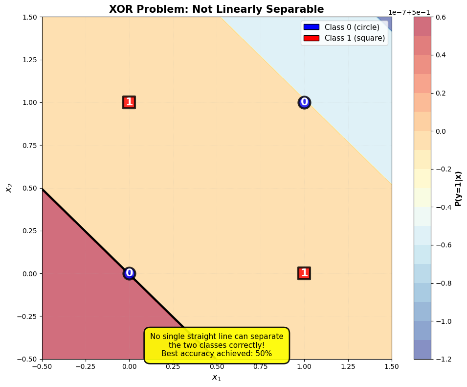

De oplossing voor het XOR-probleem (en andere niet-lineaire problemen) is om meerdere perceptrons te combineren.

References¶

Rosenblatt, F. (1958). The perceptron: A probabilistic model for information storage and organization in the brain. Psychological Review, 65(6), 386–408. 10.1037/h0042519