We zagen dat het perceptron-model (en bijgevolg ook het logistische regressiemodel) fundamentele problemen heeft om niet-lineair scheidbare problemen op te lossen. Een specifieke remedie is om meerdere perceptrons samen te voegen. Dit brengt ons bij neurale netwerken. In het geval van zogenaamde multi layer perceptrons worden inputs aan meerdere perceptrons gekoppeld en worden ook één of meerdere lagen van perceptrons voorzien tussen in- en outputs: zogenaamde hidden layers.
Source
import matplotlib.pyplot as plt
import numpy as np
from matplotlib.patches import Circle, FancyArrowPatch
Source
# Visualize a simple multi-layer perceptron with 2 hidden neurons
fig, ax = plt.subplots(figsize=(16, 10))
ax.set_xlim(0, 12)
ax.set_ylim(0, 10)
ax.axis("off")

# Define positions
input_y_positions = [7, 5, 3]  # bias, x1, x2
input_x = 1.5
hidden_x = 6
hidden_y_positions = [6.5, 3.5]  # Two hidden neurons
hidden_bias_y = 9  # Bias for hidden layer
output_x = 10.5
output_y = 5  # Center output between hidden neurons

# Color scheme
input_color = "lightblue"
input_edge = "darkblue"
bias_color = "lightcoral"
bias_edge = "darkred"
hidden_color = "lightyellow"
hidden_edge = "orange"
output_color = "lightgreen"
output_edge = "darkgreen"

# Draw input nodes
input_nodes = []
for i, y_pos in enumerate(input_y_positions):
    if i == 0:
        # Bias node
        circle = Circle(
            (input_x, y_pos), 0.35, color=bias_color, ec=bias_edge, linewidth=2.5, zorder=3
        )
        ax.text(
            input_x,
            y_pos,
            "$x_1=1$",
            ha="center",
            va="center",
            fontsize=16,
            fontweight="bold",
            zorder=4,
        )
        ax.text(input_x - 0.9, y_pos, "bias", ha="center", va="center", fontsize=12, style="italic")
    else:
        # Regular input nodes
        circle = Circle(
            (input_x, y_pos), 0.35, color=input_color, ec=input_edge, linewidth=2.5, zorder=3
        )
        ax.text(
            input_x,
            y_pos,
            f"$x_{i + 1}$",
            ha="center",
            va="center",
            fontsize=16,
            fontweight="bold",
            zorder=4,
        )

    ax.add_patch(circle)
    input_nodes.append((input_x, y_pos))

# Draw hidden layer neurons (2 neurons)
hidden_neurons = []
for j, h_y in enumerate(hidden_y_positions):
    hidden_neuron = Circle(
        (hidden_x, h_y), 0.7, color=hidden_color, ec=hidden_edge, linewidth=3, zorder=3
    )
    ax.add_patch(hidden_neuron)
    hidden_neurons.append((hidden_x, h_y))

    # Add sigma symbol and activation function
    ax.text(
        hidden_x,
        h_y + 0.12,
        "Σ",
        ha="center",
        va="center",
        fontsize=22,
        fontweight="bold",
        zorder=4,
    )
    ax.text(
        hidden_x,
        h_y - 0.2,
        f"$z_{{{j + 1}}} = h_{{{j + 1}}}" + r"(\mathbf{x},\mathbf{w})" + "$",
        ha="center",
        va="center",
        fontsize=12,
        style="italic",
        zorder=4,
    )
    ax.text(
        hidden_x,
        h_y - 0.45,
        f"$\phi(z_{{{j + 1}}})$",
        ha="center",
        va="center",
        fontsize=12,
        style="italic",
        zorder=4,
    )

# Draw bias node for hidden layer (connects to output)
bias_hidden = Circle(
    (hidden_x, hidden_bias_y), 0.35, color=bias_color, ec=bias_edge, linewidth=2.5, zorder=3
)
ax.add_patch(bias_hidden)
ax.text(
    hidden_x,
    hidden_bias_y,
    "$1$",
    ha="center",
    va="center",
    fontsize=16,
    fontweight="bold",
    zorder=4,
)
ax.text(
    hidden_x - 0.7, hidden_bias_y, "bias", ha="center", va="center", fontsize=12, style="italic"
)

# Draw output node
output_neuron = Circle(
    (output_x, output_y), 0.7, color=output_color, ec=output_edge, linewidth=3, zorder=3
)
ax.add_patch(output_neuron)
ax.text(
    output_x,
    output_y + 0.12,
    "Σ",
    ha="center",
    va="center",
    fontsize=22,
    fontweight="bold",
    zorder=4,
)
ax.text(
    output_x,
    output_y - 0.2,
    "$z = h(\phi_1, \phi_2,\mathbf{w})$",
    ha="center",
    va="center",
    fontsize=12,
    style="italic",
    zorder=4,
)
ax.text(
    output_x,
    output_y - 0.45,
    "$\hat{y} = \phi(z)$",
    ha="center",
    va="center",
    fontsize=12,
    style="italic",
    zorder=4,
)
ax.text(output_x + 1.1, output_y, "output " + r"$\hat{o}$", ha="center", va="center", fontsize=12)

# Draw connections from inputs to BOTH hidden neurons
for j, (h_x, h_y) in enumerate(hidden_neurons):
    for i, (x, y) in enumerate(input_nodes):
        arrow = FancyArrowPatch(
            (x + 0.35, y),
            (h_x - 0.7, h_y),
            arrowstyle="->",
            mutation_scale=15,
            linewidth=1.5,
            color="gray",
            alpha=0.5,
            zorder=1,
        )
        ax.add_patch(arrow)

        # Add weight labels
        mid_x = (x + h_x) / 2 - 0.2
        mid_y = (y + h_y) / 2
        weight_label = f"$w^{{(1)}}_{{{i + 1},{j + 1}}}$"
        ax.text(
            mid_x,
            mid_y,
            weight_label,
            ha="center",
            va="bottom",
            fontsize=10,
            color=bias_edge if i == 0 else input_edge,
            fontweight="bold",
            bbox={
                "boxstyle": "round,pad=0.2",
                "facecolor": "white",
                "edgecolor": "none",
                "alpha": 0.8,
            },
        )

# Draw connections from hidden neurons to output
for j, (h_x, h_y) in enumerate(hidden_neurons):
    arrow = FancyArrowPatch(
        (h_x + 0.7, h_y),
        (output_x - 0.7, output_y),
        arrowstyle="->",
        mutation_scale=15,
        linewidth=2,
        color="gray",
        alpha=0.7,
        zorder=2,
    )
    ax.add_patch(arrow)

    # Add weight labels
    mid_x = (h_x + output_x) / 2
    mid_y = (h_y + output_y) / 2
    ax.text(
        mid_x,
        mid_y,
        f"$w^{{(2)}}_{{{j + 2}}}$",
        ha="center",
        va="bottom" if j == 0 else "top",
        fontsize=11,
        color="darkorange",
        fontweight="bold",
        bbox={"boxstyle": "round,pad=0.3", "facecolor": "white", "edgecolor": "none", "alpha": 0.8},
    )

# Draw connection from bias to output
arrow = FancyArrowPatch(
    (hidden_x + 0.35, hidden_bias_y),
    (output_x - 0.7, output_y),
    arrowstyle="->",
    mutation_scale=15,
    linewidth=2,
    color="gray",
    alpha=0.7,
    zorder=2,
)
ax.add_patch(arrow)

# Add weight label for bias to output
mid_x = (hidden_x + output_x) / 2
mid_y = (hidden_bias_y + output_y) / 2 + 0.3
ax.text(
    mid_x,
    mid_y,
    "$w^{{(2)}}_{{1}}$",
    ha="center",
    va="bottom",
    fontsize=11,
    color=bias_edge,
    fontweight="bold",
    bbox={"boxstyle": "round,pad=0.3", "facecolor": "white", "edgecolor": "none", "alpha": 0.8},
)

# Add layer labels - all at y = 9.7 for alignment
layer_label_y = 9.7
ax.text(
    input_x,
    layer_label_y,
    "Input Layer",
    ha="center",
    va="center",
    fontsize=14,
    fontweight="bold",
    bbox={
        "boxstyle": "round,pad=0.5",
        "facecolor": "lightblue",
        "edgecolor": "darkblue",
        "linewidth": 2,
        "alpha": 0.9,
    },
)
ax.text(
    hidden_x,
    layer_label_y,
    "Hidden Layer",
    ha="center",
    va="center",
    fontsize=14,
    fontweight="bold",
    bbox={
        "boxstyle": "round,pad=0.5",
        "facecolor": "lightyellow",
        "edgecolor": "orange",
        "linewidth": 2,
        "alpha": 0.9,
    },
)
ax.text(
    output_x,
    layer_label_y,
    "Output Layer",
    ha="center",
    va="center",
    fontsize=14,
    fontweight="bold",
    bbox={
        "boxstyle": "round,pad=0.5",
        "facecolor": "lightgreen",
        "edgecolor": "darkgreen",
        "linewidth": 2,
        "alpha": 0.9,
    },
)

plt.tight_layout()
plt.show()
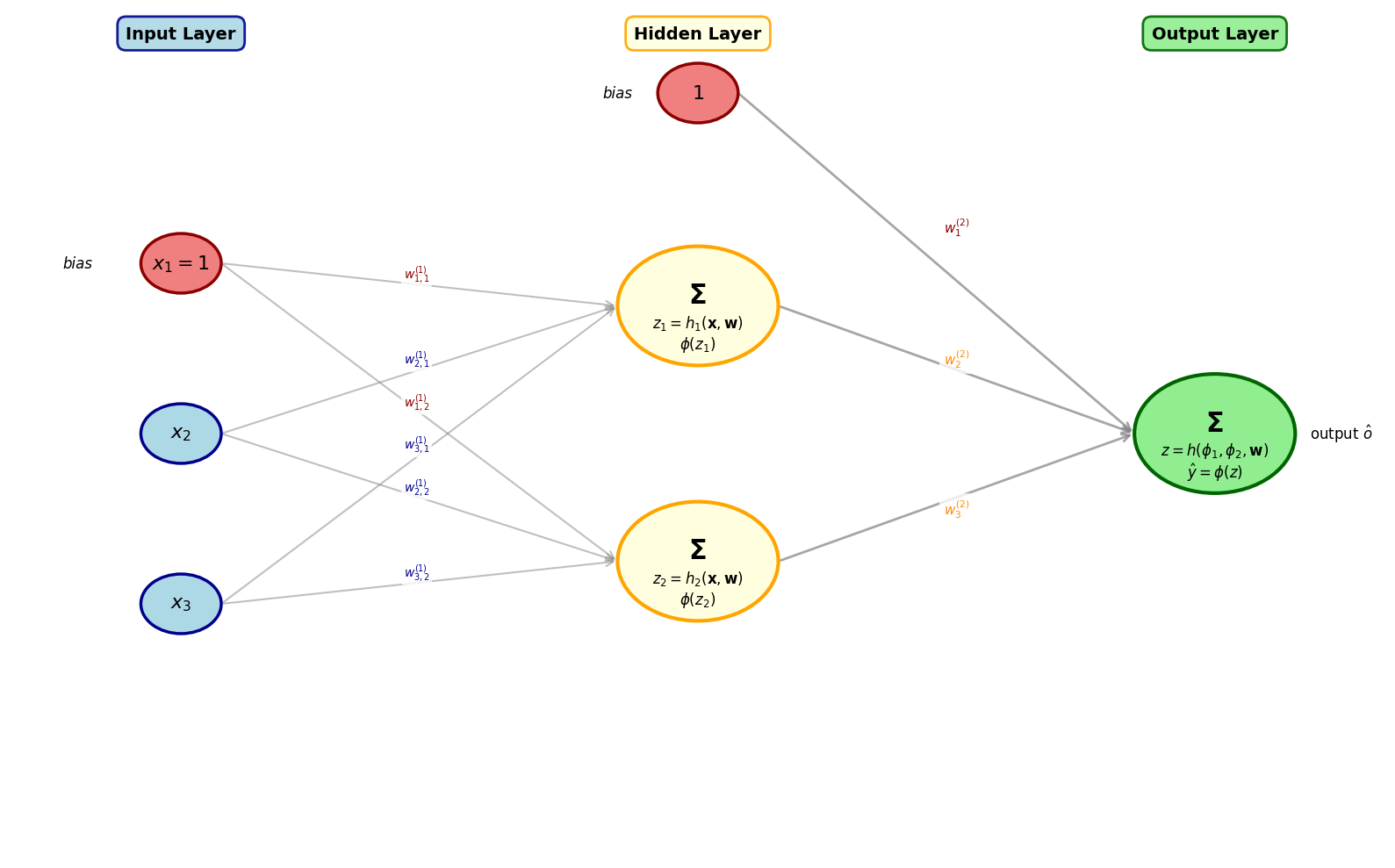
Forward pass
Iedere input wordt volgens de aanwezige connecties (architectuur) voorwaarts gepropageerd door het netwerk richting de output (van links naar rechts in bovenstaande illustratie).
In bovenstaande illustratie gaat dit als volgt:
Backward pass
Stap 1
Eens de forward pass is uitgevoerd, kunnen we de predictiefout aan de hand van de gekozen loss functie uitdrukken. Voor deze uiteenzetting kiezen we voor de squared error . Merk op dat:
we het subscript achterwege laten
we geen sum of squared errors gebruiken (zoals eerder bij het lineaire regressiemodel) omdat het hier maar over één input gaat.
we de term toevoegen omdat we hiermee de exponent wegwerken bij het berekenen van de gradiënt.
We werken ook met de veronderstelling van een logistische activatiefunctie.
We willen opnieuw via gradient descent, stap voor stap de gewichten updaten aan de hand van de partiële afgeleiden (gradiënt) van de loss functie. De individuele partiële afgeleiden geven ons telkens de richting aan waarin we een bepaald gewicht (of parameter) moeten verschuiven om de grootste daling in de loss te bekomen - rekening houdend met een bepaalde stapgrootte (learning rate) en bij het constant houden van alle andere gewichten (of parameters).
Het berekenen van de gradiënt gebeurt, gezien de (variabele) netwerkstructuur, op een speciale manier waarbij er sequentieel gewerkt wordt, beginnend bij de output en eindigend bij de input (van rechts naar links in bovenstaande illustratie). Deze beweging wordt de backward pass genoemd.
Doordat de output van het netwerk tot stand komt op basis van een reeks geneste functies, speelt de kettingregel hierin een centrale rol.
Stap 2
Nadat we in de eerste stap de loss bepaald hebben, beginnen we rechts, bij de eerste gewichten die we tegenkomen vóór de output: , en in bovenstaande illustratie.
Als we de loss in termen van die gewichten uitdrukken krijgen we:
We kunnen dit zien als vier geneste functies:
met (in de veronderstelling van een logistische activatiefunctie)
Voor de partiële afgeleide van de loss functie met betrekking tot het bias gewicht krijgen we via de kettingregel:
waarbij
We krijgen dus:
Voor de partiële afgeleide van de loss functie met betrekking tot gewicht zit het enige verschil in de laatste term van de ketting:
Hiermee kunnen we exact zoals voorheen een update berekenen binnen een gradient descent iteratie:
Stap 3
Als we nu naar de gewichten op het voorgaande niveau gaan kijken, kunnen we de ketting van partiële afgeleiden simpelweg verlengen. Laten we kijken naar gewicht dat verbonden is met input en het eerste hidden neuron.
We moeten de loss nu uitdrukken als een functie van :
We hebben nu zes geneste functies:
met
De ketting wordt:
waarbij de activatie van het eerste hidden neuron is.
De eerste drie termen kennen we al uit Stap 2 🎉:
De nieuwe termen zijn:
Dit geeft ons:
Op analoge wijze kunnen we de partiële afgeleiden voor alle andere gewichten in de inputlaag berekenen. Voor bijvoorbeeld (verbonden met input en het tweede hidden neuron) krijgen we:
Algemeen principe
De gradiënt van de loss wordt achterwaarts berekend door de loss steeds dieper uit te schrijven in termen van de bewuste gewichten. Deze terugwaartse beweging is de kern van het back propagation algoritme. Het algoritme is heel efficiënt doordat de bouwstenen van de partiële afgeleiden hergebruikt kunnen worden bij veel verschillende gewichten. Eens de gradiënt berekend is, kunnen we precies zoals voorheen gradient descent toepassen op de volledige set van gewichten (of varianten zoals stochastic gradient descent):
Merk op dat bovenstaande uiteenzetting specifiek geldt voor de geïllustreerde architectuur met logistische activatie en . Het algoritme kan echter in principe omgaan met een arbitraire architectuur en afleidbare activatiefuncties. Zo zal bij diepere netwerken (meer hidden layers) ook de somregel zijn intrede doen wanneer er vanaf een bepaald gewicht meerdere paden richting de output lopen.
Source
# Visualize a deeper network showing multiple paths from input to output
fig, ax = plt.subplots(figsize=(10, 7))
ax.set_xlim(0, 14)
ax.set_ylim(0, 10)
ax.axis("off")

# Define positions for a 4-layer network (input, 2 hidden, output)
input_x = 1.5
hidden1_x = 5
hidden2_x = 9
output_x = 12.5

# Node positions
input_positions = [8, 6, 4, 2]  # 4 input nodes
hidden1_positions = [7.5, 5, 2.5]  # 3 nodes in first hidden layer
hidden2_positions = [6.5, 3.5]  # 2 nodes in second hidden layer
output_y = 5  # 1 output node

# Draw input layer
input_nodes = []
for y_pos in input_positions:
    circle = Circle((input_x, y_pos), 0.3, color="lightblue", ec="darkblue", linewidth=2, zorder=3)
    ax.add_patch(circle)
    input_nodes.append((input_x, y_pos))

# Draw first hidden layer
hidden1_nodes = []
for y_pos in hidden1_positions:
    circle = Circle(
        (hidden1_x, y_pos), 0.4, color="lightyellow", ec="orange", linewidth=2, zorder=3
    )
    ax.add_patch(circle)
    hidden1_nodes.append((hidden1_x, y_pos))

# Draw second hidden layer
hidden2_nodes = []
for y_pos in hidden2_positions:
    circle = Circle(
        (hidden2_x, y_pos), 0.4, color="lightyellow", ec="orange", linewidth=2, zorder=3
    )
    ax.add_patch(circle)
    hidden2_nodes.append((hidden2_x, y_pos))

# Draw output layer
output_node = Circle(
    (output_x, output_y), 0.4, color="lightgreen", ec="darkgreen", linewidth=2, zorder=3
)
ax.add_patch(output_node)

# Draw all connections from input to first hidden (in gray)
for inp in input_nodes:
    for h1 in hidden1_nodes:
        arrow = FancyArrowPatch(
            (inp[0] + 0.3, inp[1]),
            (h1[0] - 0.4, h1[1]),
            arrowstyle="->",
            mutation_scale=10,
            linewidth=0.8,
            color="lightgray",
            alpha=0.5,
            zorder=1,
        )
        ax.add_patch(arrow)

# Draw all connections from first hidden to second hidden (in gray)
for h1 in hidden1_nodes:
    for h2 in hidden2_nodes:
        arrow = FancyArrowPatch(
            (h1[0] + 0.4, h1[1]),
            (h2[0] - 0.4, h2[1]),
            arrowstyle="->",
            mutation_scale=10,
            linewidth=0.8,
            color="lightgray",
            alpha=0.5,
            zorder=1,
        )
        ax.add_patch(arrow)

# Draw all connections from second hidden to output (in gray)
for h2 in hidden2_nodes:
    arrow = FancyArrowPatch(
        (h2[0] + 0.4, h2[1]),
        (output_x - 0.4, output_y),
        arrowstyle="->",
        mutation_scale=10,
        linewidth=0.8,
        color="lightgray",
        alpha=0.5,
        zorder=1,
    )
    ax.add_patch(arrow)

# Highlight ONE specific path from a specific input weight to output
# Choose second input node (index 1)
highlighted_input = input_nodes[1]

# This input connects to ALL nodes in hidden layer 1
# Let's highlight paths through first and third hidden1 nodes
highlighted_h1_indices = [0, 2]  # First and third nodes

# These then connect to different nodes in hidden layer 2
# From h1[0] to both h2 nodes, and from h1[2] to both h2 nodes
highlighted_h2_indices = [0, 1]  # Both nodes in hidden2

# Highlight: Input -> Hidden1[0] -> Hidden2[0] -> Output (PATH 1)
arrow1 = FancyArrowPatch(
    (highlighted_input[0] + 0.3, highlighted_input[1]),
    (hidden1_nodes[0][0] - 0.4, hidden1_nodes[0][1]),
    arrowstyle="->",
    mutation_scale=12,
    linewidth=3,
    color="red",
    alpha=0.7,
    zorder=2,
)
ax.add_patch(arrow1)

arrow2 = FancyArrowPatch(
    (hidden1_nodes[0][0] + 0.4, hidden1_nodes[0][1]),
    (hidden2_nodes[0][0] - 0.4, hidden2_nodes[0][1]),
    arrowstyle="->",
    mutation_scale=12,
    linewidth=3,
    color="red",
    alpha=0.7,
    zorder=2,
)
ax.add_patch(arrow2)

arrow3 = FancyArrowPatch(
    (hidden2_nodes[0][0] + 0.4, hidden2_nodes[0][1]),
    (output_x - 0.4, output_y),
    arrowstyle="->",
    mutation_scale=12,
    linewidth=3,
    color="red",
    alpha=0.7,
    zorder=2,
)
ax.add_patch(arrow3)

# Highlight: Input -> Hidden1[0] -> Hidden2[1] -> Output (PATH 2)
arrow4 = FancyArrowPatch(
    (hidden1_nodes[0][0] + 0.4, hidden1_nodes[0][1]),
    (hidden2_nodes[1][0] - 0.4, hidden2_nodes[1][1]),
    arrowstyle="->",
    mutation_scale=12,
    linewidth=3,
    color="red",
    alpha=0.7,
    zorder=2,
)
ax.add_patch(arrow4)

arrow5 = FancyArrowPatch(
    (hidden2_nodes[1][0] + 0.4, hidden2_nodes[1][1]),
    (output_x - 0.4, output_y),
    arrowstyle="->",
    mutation_scale=12,
    linewidth=3,
    color="red",
    alpha=0.7,
    zorder=2,
)
ax.add_patch(arrow5)

plt.tight_layout()
plt.show()
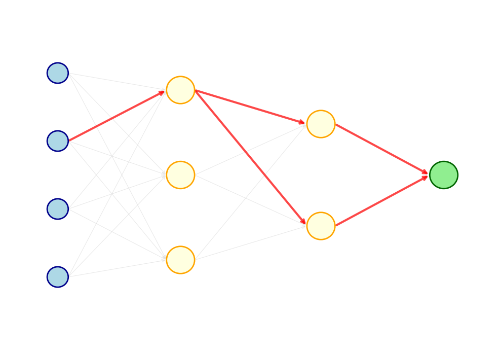
Een mogelijk probleem bij back propagation in diepe netwerken is dat bij het terug propageren van de loss, partiële afgeleiden steeds kleiner worden. Daardoor leren vroegere lagen trager dan latere lagen, wat tot leerproblemen leidt. Dit is het zogenaamde vanishing gradients probleem. Er bestaan verschillende strategieën om dit tegen te gaan, zoals de keuze voor ReLU als activatiefunctie en adaptieve learning rates (zie bijvoorbeeld het Adam optimalisatiealgoritme).