Tot nu toe hebben we gezien hoe een perceptron met een sigmoïde activatiefunctie gebruikt kan worden voor binaire klassificatie. We zagen ook hoe multi-layer perceptrons complexere beslissingsgrenzen kunnen leren door meerdere lagen van neuronen te combineren.
Maar wat als we meer dan twee klassen hebben? Bijvoorbeeld: het voorspellen van handgeschreven cijfers (0-9) of het herkennen van verschillende diersoorten in afbeeldingen?
Softmax activatiefunctie
Voor binaire klassificatie gebruiken we typisch één output neuron met een logistische activatiefunctie. De output van dat neuron ligt tussen 0 en 1. We interpreteren dit als een conditionele kans . Door een decision boundary te kiezen, wordt de eigenlijke output binair.
Voor multi-class classificatie met klassen hebben we een andere aanpak nodig:
we voorzien output neuronen: één voor elke klasse
de waarde van elke output-neuron stelt opnieuw een conditionele kans voor:
om een geldige kansverdeling te bekomen, moet de som van alle outputs moet 1 zijn
Dit is precies wat de softmax activatiefunctie doet.
De softmax functie transformeert een vector van reële getallen naar een kansverdeling:
De softmax activatiefunctie past dus de exponentiële functie toe op elk element en normaliseert vervolgens door te delen door de som van alle exponentiële waarden.
Hierdoor liggen alle outputs tussen 0 en 1, is de som van alle outputs exact 1 en krijgen hogere waarden hogere kansen. De softmax is een generalisatie van de logistische activatiefunctie naar meerdere dimensies
Gebruik:
Voor een input produceert het netwerk outputs (of logits)
Na softmax activatie: voor elke klasse
Predictie: kies de klasse met de hoogste waarschijnlijkheid
Source
import matplotlib.pyplot as plt
from matplotlib.patches import Circle, FancyArrowPatch
Source
# Visualize a multi-layer perceptron with softmax output (3 classes)
fig, ax = plt.subplots(figsize=(16, 12))
ax.set_xlim(0, 14)
ax.set_ylim(0, 11)
ax.axis("off")

# Define positions
input_y_positions = [8, 6, 4]  # bias, x1, x2
input_x = 1.5
hidden_x = 6
hidden_y_positions = [7.5, 4.5]  # Two hidden neurons
hidden_bias_y = 10  # Bias for hidden layer
logits_x = 9.5
output_x = 12.5

# 3 output classes
num_classes = 3
output_y_positions = [8, 5.5, 3]  # Three output neurons

# Color scheme
input_color = "lightblue"
input_edge = "darkblue"
bias_color = "lightcoral"
bias_edge = "darkred"
hidden_color = "lightyellow"
hidden_edge = "orange"
logits_color = "lavender"
logits_edge = "purple"
output_color = "lightgreen"
output_edge = "darkgreen"

# Draw input nodes
input_nodes = []
for i, y_pos in enumerate(input_y_positions):
    if i == 0:
        # Bias node
        circle = Circle(
            (input_x, y_pos), 0.35, color=bias_color, ec=bias_edge, linewidth=2.5, zorder=3
        )
        ax.text(
            input_x,
            y_pos,
            "$x_1=1$",
            ha="center",
            va="center",
            fontsize=16,
            fontweight="bold",
            zorder=4,
        )
        ax.text(input_x - 0.9, y_pos, "bias", ha="center", va="center", fontsize=12, style="italic")
    else:
        # Regular input nodes
        circle = Circle(
            (input_x, y_pos), 0.35, color=input_color, ec=input_edge, linewidth=2.5, zorder=3
        )
        ax.text(
            input_x,
            y_pos,
            f"$x_{i + 1}$",
            ha="center",
            va="center",
            fontsize=16,
            fontweight="bold",
            zorder=4,
        )

    ax.add_patch(circle)
    input_nodes.append((input_x, y_pos))

# Draw hidden layer neurons (2 neurons)
hidden_neurons = []
for j, h_y in enumerate(hidden_y_positions):
    hidden_neuron = Circle(
        (hidden_x, h_y), 0.7, color=hidden_color, ec=hidden_edge, linewidth=3, zorder=3
    )
    ax.add_patch(hidden_neuron)
    hidden_neurons.append((hidden_x, h_y))

    # Add sigma symbol and activation function
    ax.text(
        hidden_x,
        h_y + 0.12,
        "Σ",
        ha="center",
        va="center",
        fontsize=22,
        fontweight="bold",
        zorder=4,
    )
    ax.text(
        hidden_x,
        h_y - 0.2,
        f"$\phi(z_{{{j + 1}}})$",
        ha="center",
        va="center",
        fontsize=12,
        style="italic",
        zorder=4,
    )

# Draw bias node for hidden layer (connects to output)
bias_hidden = Circle(
    (hidden_x, hidden_bias_y), 0.35, color=bias_color, ec=bias_edge, linewidth=2.5, zorder=3
)
ax.add_patch(bias_hidden)
ax.text(
    hidden_x,
    hidden_bias_y,
    "$1$",
    ha="center",
    va="center",
    fontsize=16,
    fontweight="bold",
    zorder=4,
)
ax.text(
    hidden_x - 0.7, hidden_bias_y, "bias", ha="center", va="center", fontsize=12, style="italic"
)

# Draw connections from inputs to BOTH hidden neurons
for j, (h_x, h_y) in enumerate(hidden_neurons):
    for i, (x, y) in enumerate(input_nodes):
        arrow = FancyArrowPatch(
            (x + 0.35, y),
            (h_x - 0.7, h_y),
            arrowstyle="->",
            mutation_scale=15,
            linewidth=1.5,
            color="gray",
            alpha=0.5,
            zorder=1,
        )
        ax.add_patch(arrow)

        # Add weight labels
        mid_x = (x + h_x) / 2 - 0.2
        mid_y = (y + h_y) / 2
        weight_label = f"$w^{{(1)}}_{{{i + 1},{j + 1}}}$"
        ax.text(
            mid_x,
            mid_y,
            weight_label,
            ha="center",
            va="bottom",
            fontsize=10,
            color=bias_edge if i == 0 else input_edge,
            fontweight="bold",
            bbox={
                "boxstyle": "round,pad=0.2",
                "facecolor": "white",
                "edgecolor": "none",
                "alpha": 0.8,
            },
        )

# Draw logits layer (K output neurons before softmax)
logits_neurons = []
for k, out_y in enumerate(output_y_positions):
    logit_neuron = Circle(
        (logits_x, out_y), 0.6, color=logits_color, ec=logits_edge, linewidth=3, zorder=3
    )
    ax.add_patch(logit_neuron)
    logits_neurons.append((logits_x, out_y))

    # Add sigma symbol
    ax.text(
        logits_x,
        out_y + 0.05,
        "Σ",
        ha="center",
        va="center",
        fontsize=20,
        fontweight="bold",
        zorder=4,
    )
    # Add logit label
    ax.text(
        logits_x,
        out_y - 0.25,
        f"$z_{k + 1}$",
        ha="center",
        va="center",
        fontsize=12,
        style="italic",
        zorder=4,
    )

# Draw connections from hidden neurons to ALL logits
for k, (l_x, l_y) in enumerate(logits_neurons):
    for j, (h_x, h_y) in enumerate(hidden_neurons):
        arrow = FancyArrowPatch(
            (h_x + 0.7, h_y),
            (l_x - 0.6, l_y),
            arrowstyle="->",
            mutation_scale=15,
            linewidth=1.5,
            color="gray",
            alpha=0.5,
            zorder=2,
        )
        ax.add_patch(arrow)

        # Add weight labels
        mid_x = (h_x + l_x) / 2
        mid_y = (h_y + l_y) / 2
        ax.text(
            mid_x,
            mid_y,
            f"$w^{{(2)}}_{{{j + 2},{k + 1}}}$",
            ha="center",
            va="bottom",
            fontsize=9,
            color="darkorange",
            fontweight="bold",
            bbox={
                "boxstyle": "round,pad=0.2",
                "facecolor": "white",
                "edgecolor": "none",
                "alpha": 0.8,
            },
        )

# Draw connections from bias to ALL logits
for k, (l_x, l_y) in enumerate(logits_neurons):
    arrow = FancyArrowPatch(
        (hidden_x + 0.35, hidden_bias_y),
        (l_x - 0.6, l_y),
        arrowstyle="->",
        mutation_scale=15,
        linewidth=1.5,
        color="gray",
        alpha=0.5,
        zorder=2,
    )
    ax.add_patch(arrow)

    # Add weight label for bias to logits
    mid_x = (hidden_x + l_x) / 2 - 0.3
    mid_y = (hidden_bias_y + l_y) / 2
    ax.text(
        mid_x,
        mid_y,
        f"$w^{{(2)}}_{{1,{k + 1}}}$",
        ha="center",
        va="bottom",
        fontsize=9,
        color=bias_edge,
        fontweight="bold",
        bbox={"boxstyle": "round,pad=0.2", "facecolor": "white", "edgecolor": "none", "alpha": 0.8},
    )

# Draw softmax output nodes
for k, out_y in enumerate(output_y_positions):
    output_neuron = Circle(
        (output_x, out_y), 0.6, color=output_color, ec=output_edge, linewidth=3, zorder=3
    )
    ax.add_patch(output_neuron)

    # Add probability label
    ax.text(
        output_x,
        out_y,
        f"$\\hat{{y}}_{k + 1} = P(\\hat{{o}}_{k + 1}=1)$",
        ha="center",
        va="center",
        fontsize=13,
        fontweight="bold",
        zorder=4,
    )

    # Add y-hat label
    ax.text(
        output_x + 0.9,
        out_y,
        f"$\\hat{{o}}_{k + 1}$",
        ha="center",
        va="center",
        fontsize=14,
        fontweight="bold",
    )

# Draw arrows from logits to softmax outputs with softmax label
for k, ((l_x, l_y), (o_x, o_y)) in enumerate(
    zip(logits_neurons, [(output_x, y) for y in output_y_positions])
):
    arrow = FancyArrowPatch(
        (l_x + 0.6, l_y),
        (o_x - 0.6, o_y),
        arrowstyle="->",
        mutation_scale=15,
        linewidth=2.5,
        color="darkgreen",
        alpha=0.7,
        zorder=2,
    )
    ax.add_patch(arrow)

# Add softmax label in the middle
softmax_x = (logits_x + output_x) / 2
softmax_y = (max(output_y_positions) + min(output_y_positions)) / 2
ax.text(
    softmax_x,
    softmax_y,
    "softmax",
    ha="center",
    va="center",
    fontsize=16,
    fontweight="bold",
    style="italic",
    color="darkgreen",
    bbox={
        "boxstyle": "round,pad=0.5",
        "facecolor": "lightgreen",
        "edgecolor": "darkgreen",
        "linewidth": 2.5,
        "alpha": 0.9,
    },
)

# Add layer labels
layer_label_y = 10.7
ax.text(
    input_x,
    layer_label_y,
    "Input Layer",
    ha="center",
    va="center",
    fontsize=14,
    fontweight="bold",
    bbox={
        "boxstyle": "round,pad=0.5",
        "facecolor": "lightblue",
        "edgecolor": "darkblue",
        "linewidth": 2,
        "alpha": 0.9,
    },
)
ax.text(
    hidden_x,
    layer_label_y,
    "Hidden Layer",
    ha="center",
    va="center",
    fontsize=14,
    fontweight="bold",
    bbox={
        "boxstyle": "round,pad=0.5",
        "facecolor": "lightyellow",
        "edgecolor": "orange",
        "linewidth": 2,
        "alpha": 0.9,
    },
)
ax.text(
    logits_x,
    layer_label_y,
    "Linear Outputs",
    ha="center",
    va="center",
    fontsize=14,
    fontweight="bold",
    bbox={
        "boxstyle": "round,pad=0.5",
        "facecolor": "lavender",
        "edgecolor": "purple",
        "linewidth": 2,
        "alpha": 0.9,
    },
)
ax.text(
    output_x,
    layer_label_y,
    "Output Layer",
    ha="center",
    va="center",
    fontsize=14,
    fontweight="bold",
    bbox={
        "boxstyle": "round,pad=0.5",
        "facecolor": "lightgreen",
        "edgecolor": "darkgreen",
        "linewidth": 2,
        "alpha": 0.9,
    },
)

# Add title
ax.text(
    7,
    0.5,
    "Multi-class Neural Network with Softmax Activation",
    ha="center",
    va="center",
    fontsize=16,
    fontweight="bold",
)

plt.tight_layout()
plt.show()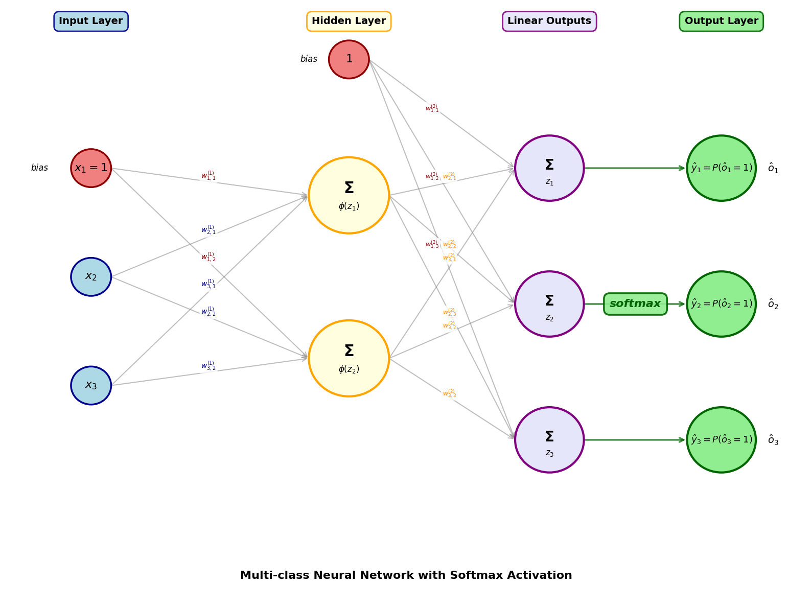
Implicaties voor gradiëntberekening
De softmax activatiefunctie heeft belangrijke gevolgen voor de backward pass tijdens het trainen van het netwerk:
Gekoppelde outputs
In tegenstelling tot de logistische activatiefunctie, waarbij elk neuron onafhankelijk geactiveerd wordt, zijn de softmax outputs onderling afhankelijk. De output van één neuron beïnvloedt alle andere outputs door de normalisatie. Dit betekent dat bij het berekenen van de gradiënt met betrekking tot een bepaald , alle softmax outputs een rol spelen.
Partiële afgeleiden
Voor de partiële afgeleide van softmax output naar logit geldt:
Deze formule toont dat:
De diagonale termen () lijken op de afgeleide van de logistische functie:
De off-diagonale termen () zijn negatief en koppelen verschillende outputs aan elkaar
Cross-entropy loss
In de praktijk wordt softmax bijna altijd gecombineerd met de categorical cross-entropy loss functie:
waarbij de one-hot encoded target is (dus voor de juiste klasse en voor alle andere klassen).
Een elegante eigenschap van deze combinatie is dat de gradiënt van de loss naar de logits zeer eenvoudig wordt:
Dit is de voorspelde kans minus de werkelijke target. Deze eenvoudige vorm maakt de backward pass efficiënt en numeriek stabiel, ondanks de complexiteit van de softmax functie zelf.