t-SNE en UMAP

Naast PCA bestaan er andere technieken voor dimensionaliteitsreductie die specifiek ontworpen zijn om lokale structuur en non-lineaire patronen te behouden. Er zijn tegenwoordig twee belangrijke alternatieven: t-SNE (t-distributed Stochastic Neighbor Embedding) en UMAP (Uniform Manifold Approximation and Projection)

Beperkingen van PCA¶

• Lineaire projectie: Kan alleen lineaire relaties vastleggen

• Globale focus: Maximaliseert variantie, maar behoudt lokale structuur niet noodzakelijk

• Euclidische afstanden: Werkt minder goed bij bepaalde structuren

t-SNE¶

Intuïtie¶

t-SNE (t-distributed Stochastic Neighbor Embedding) bewaart lokale nabijheden door punten die dicht bij elkaar liggen in de hoge-dimensionale ruimte ook dicht bij elkaar te houden in de lage-dimensionale visualisatie.

Kernidee: Converteer afstanden naar waarschijnlijkheden

1. In de originele hoge dimensies: Voor elk punt $\mathbf{x}_i$, bereken de waarschijnlijkheid dat het punt $\mathbf{x}_j$ als “buur” kiest:

   $$p_{j|i} = \frac{\exp(-\|\mathbf{x}_i - \mathbf{x}_j\|^2 / 2\sigma_i^2)}{\sum_{k \neq i} \exp(-\|\mathbf{x}_i - \mathbf{x}_k\|^2 / 2\sigma_i^2)}$$

   (1)

   Dit is een Normaalverdeling: punten die dicht bij $\mathbf{x}_i$ liggen krijgen een hoge waarschijnlijkheid.

2. In de target lage dimensies: Definieer analoge waarschijnlijkheden $q_{ij}$ voor de lage-dimensionale punten $\mathbf{y}_i$, maar nu met een t-distributie (Student-t met 1 vrijheidsgraad):

   $$q_{ij} = \frac{(1 + \|\mathbf{y}_i - \mathbf{y}_j\|^2)^{-1}}{\sum_{k \neq l}(1 + \|\mathbf{y}_k - \mathbf{y}_l\|^2)^{-1}}$$

   (2)

   De t-distributie heeft zwaardere staarten dan een Normaalverdeling, wat helpt om het crowding problem op te lossen (in lage dimensies is er minder ruimte voor alle punten).

3. Optimalisatie: Vind $\mathbf{y}_i$ die de Kullback-Leibler divergentie tussen $P$ en $Q$ minimaliseert:

   $$\text{KL}(P\|Q) = \sum_{i,j} p_{ij} \log \frac{p_{ij}}{q_{ij}}$$

   (3)

   Intuïtief: straf situaties waar $p_{ij}$ groot is (punten zijn buren in hoge dimensies) maar $q_{ij}$ klein is (ver uit elkaar in visualisatie).

Voordelen¶

• Excellente clustering: Onthult natuurlijke clusters zeer duidelijk

• Lokale structuur: Behoudt de nabijheid van vergelijkbare punten

• Niet-lineair: Kan complexe manifold-structuren vastleggen

Beperkingen¶

• Geen globale structuur: Afstanden tussen clusters zijn niet betekenisvol

• Computationeel zwaar: $O(n^2)$ complexiteit (maar algoritmes zoals Barnes-Hut reduceren dit)

• Niet-deterministisch: Resultaat hangt af van initialisatie en hyperparameters

• Geen nieuwe data: Geen directe transformatie voor nieuwe punten (wel approximaties)

UMAP¶

Intuïtie¶

UMAP (Uniform Manifold Approximation and Projection) is gebaseerd op de assumptie dat data op een lager-dimensionale manifold ligt in de hoge-dimensionale ruimte. Het gebruikt ideeën uit Riemannse meetkunde en topologie.

Kernidee: Bouw een graafrepresentatie van de data

1. Lokale afstandsmetriek: UMAP veronderstelt dat de data lokaal Euclidisch is. Voor elk punt $\mathbf{x}_i$ schatten we de lokale metriek door de afstand tot de dichtstbijzijnde buur $\rho_i$:

   $$w(\mathbf{x}_i, \mathbf{x}_j) = \exp\left(-\frac{\max(0, d(\mathbf{x}_i, \mathbf{x}_j) - \rho_i)}{\sigma_i}\right)$$

   (4)

   waar $d(\mathbf{x}_i, \mathbf{x}_j)$ de afstand tussen punten is. Dit creëert een fuzzy graph waar edges gewichten hebben tussen 0 en 1.

2. Fuzzy simplicial complex: De gewichten $w(\mathbf{x}_i, \mathbf{x}_j)$ definiëren een topologische structuur:

   • Punt $j$ behoort “gedeeltelijk” tot de buurt van punt $i$

   • Symmetriseer: $w_{ij} = w(\mathbf{x}_i, \mathbf{x}_j) + w(\mathbf{x}_j, \mathbf{x}_i) - w(\mathbf{x}_i, \mathbf{x}_j) \cdot w(\mathbf{x}_j, \mathbf{x}_i)$

3. Optimalisatie: Vind lage-dimensionale representatie met analoge graaf $V$ die $W$ benadert via cross-entropy:

   $$\mathcal{L} = \sum_{i,j} w_{ij} \log \frac{w_{ij}}{v_{ij}} + (1-w_{ij})\log\frac{1-w_{ij}}{1-v_{ij}}$$

   (5)

   Dit balanceert:

   • Aantrekking: Als $w_{ij}$ hoog is (buren), maak $v_{ij}$ ook hoog

   • Afstoting: Als $w_{ij}$ laag is (geen buren), maak $v_{ij}$ ook laag

Sleutelverschil met t-SNE: UMAP bewaart meer globale structuur door de manifold-assumptie en fuzzy topologie.

Voordelen¶

• Sneller dan t-SNE: $O(n)$ in plaats van $O(n^2)$, schaalbaar naar miljoenen punten

• Globale + lokale structuur: Behoudt zowel clusters als hun onderlinge posities

• Generaliseerbaar: Kan nieuwe data transformeren zonder opnieuw trainen

• Flexibel: Werkt goed voor verschillende $n_{\text{components}}$ (niet alleen 2D)

Beperkingen¶

• Hyperparameters: Gevoelig voor n_neighbors en min_dist

• Theoretische basis: Complexere wiskunde, minder intuïtief dan PCA

• Interpretatie: Afstanden in lage dimensies zijn niet direct Euclidisch

PCA vs t-SNE vs UMAP¶

Vuistregels voor keuze¶

PCA¶

• Data is ongeveer lineair

• Je wilt snelle, schaalbare dimensionaliteitsreductie

• Je wilt interpreteerbare componenten

• Je moet nieuwe data kunnen transformeren

t-SNE¶

• Visualisatie is het hoofddoel

• Je wilt duidelijke clusterseparatie

• Dataset is niet te groot (< 10.000 punten)

• Lokale structuur is belangrijker dan globale

UMAP¶

• Je wilt zowel clusters als hun onderlinge relaties

• Dataset is groot (> 10.000 punten)

• Je moet nieuwe data kunnen transformeren

• Je wilt verder werken met de embedding (niet alleen visualisatie)

Praktische toepassing¶

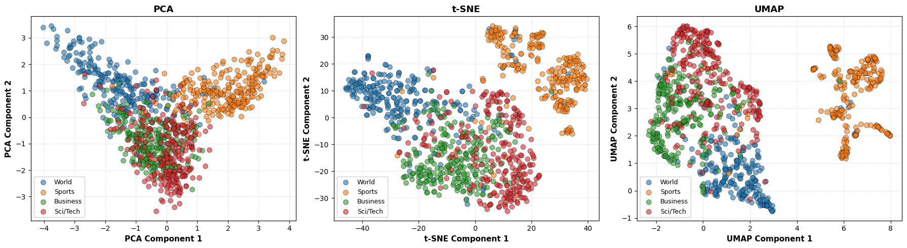
We gebruiken dezelfde AG News dataset met BERT embeddings als in het PCA notebook, maar nu vergelijken we PCA, t-SNE en UMAP naast elkaar. Dit laat zien hoe verschillende technieken dezelfde hoog-dimensionale data (768D) anders visualiseren.