Als alternatief voor grid search zouden we via sampling kunnen werken.
We starten met een eerste berekende gok voor de parameters en berekenen de loss bij de start
Daarna itereren we (30k keer) over volgende stappen:
We nemen een sample uit een normale verdeling met gemiddelde 0 om een kleine aanpassing te doen aan de parameterschattingen (in positieve of negatieve zin).
We zorgen dat de bijgewerkte schattingen binnen een realistisch interval blijven.
We berekenen de loss opnieuw. Als de nieuwe is gedaald, behouden we de nieuwe parameterwaarden. In het andere geval verwerpen we ze.
Source
import matplotlib.pyplot as plt
import numpy as np

from ml_courses.sim.monte_carlo_tips import MonteCarloTipsSimulation
Source
# Generate data
sim = MonteCarloTipsSimulation()

# Random number generator for reproducibility
rng = np.random.default_rng(67)

# Standardized variables
order_totals = (sim.order_totals - np.mean(sim.order_totals)) / np.std(sim.order_totals)
observed_tips = (sim.observed_tips - np.mean(sim.observed_tips)) / np.std(sim.observed_tips)

# Initial guesses
b1 = rng.uniform(-2.0, 2.0)
b2 = rng.uniform(-1.0, 3.0)

# Initial SSE loss
current_loss = sim.calculate_loss(b1, b2, order_totals, observed_tips)
print(
    f"Current SSE loss: {current_loss:.2f} (with guess: {b1:.2f} + {b2:.2f} × standardized_order)"
)

# Containers to keep track of all our attempts
b1_samples = []
b2_samples = []
loss_samples = []

n_accepted = 0  # Count how many proposals we accepted
n_samples = 30000  # Total number of samples to draw
step_size = 0.0001  # How big of a step to take when proposing new

for i in range(n_samples):
    # Propose slight changes to our current best guess
    b1_new = b1 + rng.normal(0, step_size * 5)  # Base tip can vary more
    b2_new = b2 + rng.normal(0, step_size)

    # Keep parameters reasonable (tip rate: 0-50%, base tip: $0-5)
    b1_new = np.clip(b1_new, 0, 50)
    b2_new = np.clip(b2_new, 0, 1.0)

    new_loss = sim.calculate_loss(b1_new, b2_new, order_totals, observed_tips)

    # Decide whether this new relationship is worth keeping
    accept = False
    if new_loss < current_loss:
        # This predicts tips better - definitely keep it!
        accept = True

    if accept:
        b1 = b1_new
        b2 = b2_new
        current_loss = new_loss
        n_accepted += 1

    # Record our current best guess (whether we moved or stayed)
    b1_samples.append(b1)
    b2_samples.append(b2)
    loss_samples.append(current_loss)

    # Show progress
    if i == 0 or (i + 1) % 1000 == 0:
        tip_pct = b2 * 100
        print(
            f"Sample {i + 1:5d}: Standardized Tip = {b1:.2f} + {b2:.2f} × Standardized Order Total, loss={current_loss:.1f}"
        )

acceptance_rate = n_accepted / n_samples
print(f"\n✅ Finished! Accepted {acceptance_rate:.1%} of proposed changes")
Current SSE loss: 115.68 (with guess: -0.34 + -0.49 × standardized_order)
Sample 1: Standardized Tip = 0.00 + 0.00 × Standardized Order Total, loss=50.0
Sample 1000: Standardized Tip = 0.00 + 0.04 × Standardized Order Total, loss=46.2
Sample 2000: Standardized Tip = 0.00 + 0.08 × Standardized Order Total, loss=42.8
Sample 3000: Standardized Tip = 0.00 + 0.12 × Standardized Order Total, loss=39.3
Sample 4000: Standardized Tip = 0.00 + 0.16 × Standardized Order Total, loss=35.8
Sample 5000: Standardized Tip = 0.01 + 0.20 × Standardized Order Total, loss=32.8
Sample 6000: Standardized Tip = 0.00 + 0.24 × Standardized Order Total, loss=29.8
Sample 7000: Standardized Tip = 0.01 + 0.28 × Standardized Order Total, loss=27.0
Sample 8000: Standardized Tip = 0.01 + 0.32 × Standardized Order Total, loss=24.4
Sample 9000: Standardized Tip = 0.01 + 0.35 × Standardized Order Total, loss=21.9
Sample 10000: Standardized Tip = 0.01 + 0.40 × Standardized Order Total, loss=19.5
Sample 11000: Standardized Tip = 0.00 + 0.44 × Standardized Order Total, loss=17.3
Sample 12000: Standardized Tip = 0.00 + 0.47 × Standardized Order Total, loss=15.3
Sample 13000: Standardized Tip = 0.00 + 0.51 × Standardized Order Total, loss=13.5
Sample 14000: Standardized Tip = 0.00 + 0.55 × Standardized Order Total, loss=11.7
Sample 15000: Standardized Tip = 0.00 + 0.59 × Standardized Order Total, loss=10.1
Sample 16000: Standardized Tip = 0.00 + 0.63 × Standardized Order Total, loss=8.7
Sample 17000: Standardized Tip = 0.00 + 0.67 × Standardized Order Total, loss=7.4
Sample 18000: Standardized Tip = 0.00 + 0.71 × Standardized Order Total, loss=6.4
Sample 19000: Standardized Tip = 0.00 + 0.75 × Standardized Order Total, loss=5.5
Sample 20000: Standardized Tip = 0.00 + 0.79 × Standardized Order Total, loss=4.7
Sample 21000: Standardized Tip = 0.00 + 0.83 × Standardized Order Total, loss=4.1
Sample 22000: Standardized Tip = 0.00 + 0.86 × Standardized Order Total, loss=3.6
Sample 23000: Standardized Tip = 0.00 + 0.90 × Standardized Order Total, loss=3.3
Sample 24000: Standardized Tip = 0.00 + 0.94 × Standardized Order Total, loss=3.1
Sample 25000: Standardized Tip = 0.00 + 0.97 × Standardized Order Total, loss=3.1
Sample 26000: Standardized Tip = 0.00 + 0.97 × Standardized Order Total, loss=3.1
Sample 27000: Standardized Tip = 0.00 + 0.97 × Standardized Order Total, loss=3.1
Sample 28000: Standardized Tip = 0.00 + 0.97 × Standardized Order Total, loss=3.1
Sample 29000: Standardized Tip = 0.00 + 0.97 × Standardized Order Total, loss=3.1
Sample 30000: Standardized Tip = 0.00 + 0.97 × Standardized Order Total, loss=3.1
✅ Finished! Accepted 40.8% of proposed changes
Visualisatie van het oppervlak
Nu we de Monte Carlo sampling hebben uitgevoerd, kunnen we stappen visualiseren op het oppervlak. Zo zien we hoe het algoritme “bergafwaarts” beweegt naar het minimum.
Source
from ml_courses.sim.linear_regression_sse_viz import LinearRegressionSSEVisualizer

viz = LinearRegressionSSEVisualizer(
    x_data=sim.order_totals,
    y_data=sim.observed_tips,
    true_bias=sim.true_b1,
    true_slope=sim.true_b2,
    standardize=True,
)

fig = viz.create_3d_surface_plot(
    bias_samples=np.array(b1_samples),
    slope_samples=np.array(b2_samples),
    loss_samples=np.array(loss_samples),
    resolution=40,
    scale_factor=1.1,
)
fig.show()Hieronder herhalen we het naïeve Monte Carlo algorithme 10 keer en visualiseren we de resulterende regressielijnen.
Source
b1_sims = []
b2_sims = []

for _ in range(10):
    sim_run = sim.run_simulation(
        n_samples=15000,
        step_size=0.0001,
        b1_init=rng.uniform(-2.0, 2.0),
        b2_init=rng.uniform(-1.0, 3.0),
        b1_bounds=(-10, 10),
        b2_bounds=(-8, 10),
        order_totals=order_totals,
        observed_tips=observed_tips,
    )
    print(
        f"Estimated relationship: Standardized Tip = {sim_run['final_b1']:.2f} + {sim_run['final_b2']:.2f} × Standardized Order Total"
    )
    b1_sims.append(sim_run["final_b1"])
    b2_sims.append(sim_run["final_b2"])
Estimated relationship: Standardized Tip = 0.00 + 0.55 × Standardized Order Total
Estimated relationship: Standardized Tip = 0.00 + -0.13 × Standardized Order Total
Estimated relationship: Standardized Tip = 0.01 + 2.30 × Standardized Order Total
Estimated relationship: Standardized Tip = 0.00 + 0.53 × Standardized Order Total
Estimated relationship: Standardized Tip = 0.02 + 2.25 × Standardized Order Total
Estimated relationship: Standardized Tip = 0.00 + 2.15 × Standardized Order Total
Estimated relationship: Standardized Tip = -0.00 + 0.53 × Standardized Order Total
Estimated relationship: Standardized Tip = 0.00 + 0.93 × Standardized Order Total
Estimated relationship: Standardized Tip = -0.01 + 2.30 × Standardized Order Total
Estimated relationship: Standardized Tip = -0.00 + 0.95 × Standardized Order Total
Source
# Plot the simulations
plt.figure(figsize=(12, 6))
plt.scatter(
    sim.order_totals,
    sim.observed_tips,
    alpha=0.7,
    color="saddlebrown",
    s=60,
    edgecolor="white",
    linewidth=0.5,
    label="Customer tips",
)

true_b1 = (
    sim.true_b1 + sim.true_b2 * np.mean(sim.order_totals) - np.mean(sim.observed_tips)
) / np.std(sim.observed_tips)
true_b2 = sim.true_b2 * (np.std(sim.order_totals) / np.std(sim.observed_tips))
true_tips = sim.true_b1 + sim.true_b2 * sim.order_totals
plt.plot(
    sim.order_totals,
    true_tips,
    "r--",
    linewidth=2,
    label=f"True relationship ({true_b1:.2f} + {true_b2:.2f} × Standardized Order Total)",
)

colors = [
    "tab:blue",
    "tab:orange",
    "tab:green",
    "tab:red",
    "tab:purple",
    "tab:brown",
    "tab:pink",
    "tab:gray",
    "tab:olive",
    "tab:cyan",
]

for i, (b1_sim, b2_sim) in enumerate(zip(b1_sims, b2_sims, strict=False)):
    sim_tips = b1_sim + b2_sim * order_totals
    sim_tips = sim_tips * np.std(sim.observed_tips) + np.mean(sim.observed_tips)
    plt.plot(
        sim.order_totals,
        sim_tips,
        color=colors[i],
        linestyle="-",
        alpha=0.3,
        linewidth=1,
        label=f"MC {i + 1}: {b1_sim:.2f} + {b2_sim:.2f} × Standardized Order Total",
    )

plt.xlabel("Order Total ($)")
plt.ylabel("Tip Amount ($)")
plt.title("☕ Order Size vs Tips")
plt.legend(bbox_to_anchor=(1.05, 1), loc="upper left")
plt.grid(True, alpha=0.3)
plt.tight_layout()
plt.show()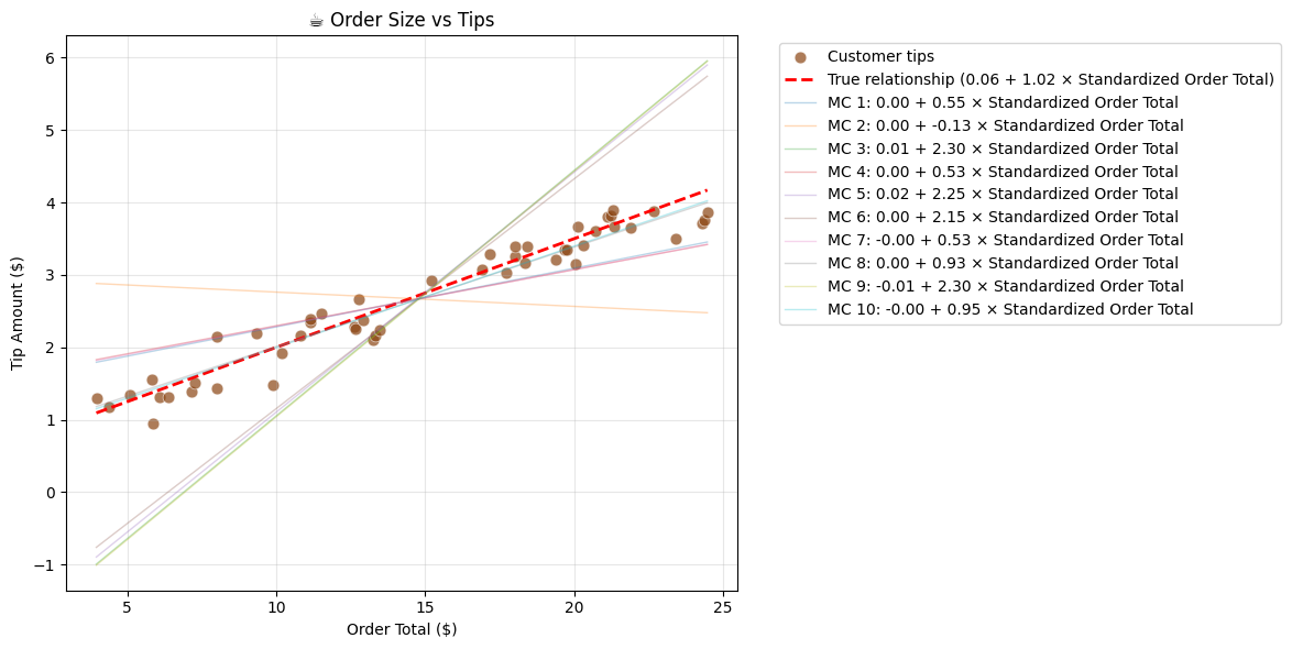
De simpele Monte Carlo benadering levert duidelijk onstabiele resultaten op. In de volgende secties bekijken we betere alternatieven op basis van calculus. Daarvoor behandelen we eerst het concept van de gradiënt van de loss functie.